In this linear algebra tutorial, we will learn how to calculate eigenvalues and eigenvectors of matrices by hand. It is true that today almost all calculations are done by using computers. However, knowing how to calculate a linear algebra object or a quantity by hand is very important since only in that way we can truly obtain a long-lasting and solid understanding of numerical linear algebra. Moreover, by learning how to compute quantities by hand, we will obtain enough insights into how linear algebra algorithms work behind the scenes. This knowledge will enable us to develop new algorithms. The YouTube video accompanying this tutorial is given below.
Definition of Eigenvalues, Eigenvectors, and Characteristic Polynomial
Let us consider an ![]() matrix
matrix ![]() .
.
Definition of eigenvalues and eigenvectors: A (complex) number ![]() is an eigenvalue of the matrix
is an eigenvalue of the matrix ![]() , if there exists a non-zero vector
, if there exists a non-zero vector ![]() such that
such that
(1) ![]()
The vector ![]() is called the eigenvector of the matrix
is called the eigenvector of the matrix ![]() .
.
Consider this equation
(2) ![]()
where ![]() is an arbitrary n-dimensional vector. We can say that the matrix
is an arbitrary n-dimensional vector. We can say that the matrix ![]() acts on the vector
acts on the vector ![]() . This means the following. Depending on the direction of
. This means the following. Depending on the direction of ![]() , the matrix
, the matrix ![]() can rotate and scale the vector. If the eigenvalue is real, then the eigenvector can be interpreted like this. The eigenvector is the vector that is only being scaled by the action of the matrix with the possibility of changing the sign! That is, if
can rotate and scale the vector. If the eigenvalue is real, then the eigenvector can be interpreted like this. The eigenvector is the vector that is only being scaled by the action of the matrix with the possibility of changing the sign! That is, if ![]() is an eigenvector and if
is an eigenvector and if ![]() is real, then if we multiply
is real, then if we multiply ![]() we will obtain
we will obtain ![]() and that is precisely the scaled version of the vector
and that is precisely the scaled version of the vector ![]() . The action line of the vector
. The action line of the vector ![]() did not change by the action of the matrix
did not change by the action of the matrix ![]() .
.
The eigenvalues can be real or complex. Here, it should also be kept in mind that the entries of eigenvectors can be complex numbers! Also, it should be observed that the eigenvector ![]() is the vector that belongs to the null space of the matrix
is the vector that belongs to the null space of the matrix ![]() .
.
Let us now explain how to compute the eigenvectors and eigenvalues. The equation (1) can be written in the equivalent form
(3) ![]()
here ![]() is
is ![]() identity matrix. We are searching for a non-zero solution
identity matrix. We are searching for a non-zero solution ![]() of this homogeneous system of equations. That is, we are searching only for non-trivial solutions. This system will have non-zero solution
of this homogeneous system of equations. That is, we are searching only for non-trivial solutions. This system will have non-zero solution ![]() if and only if the determinant of the matrix
if and only if the determinant of the matrix ![]() is equal to zero. That is, the system has non-trivial solutions if and only if
is equal to zero. That is, the system has non-trivial solutions if and only if
(4) ![]()
The equation (4) is a polynomial in ![]() . The equation (4) is called the characteristic polynomial or the characteristic equation of the matrix
. The equation (4) is called the characteristic polynomial or the characteristic equation of the matrix ![]() . The solution of the characteristic polynomial, or equivalently, its roots are the eigenvalues of the matrix
. The solution of the characteristic polynomial, or equivalently, its roots are the eigenvalues of the matrix ![]() . Generally speaking, the polynomial (4) is of order
. Generally speaking, the polynomial (4) is of order ![]() , and consequently, we will have
, and consequently, we will have ![]() eigenvalues. Note here that some eigenvalues can be identical. Let the eigenvalues be denoted by
eigenvalues. Note here that some eigenvalues can be identical. Let the eigenvalues be denoted by ![]() . Let us for the time being assume that the eigenvalues are distinct. That is, to every eigenvalue, we can associate an eigenvector. Let such eigenvectors be denoted by
. Let us for the time being assume that the eigenvalues are distinct. That is, to every eigenvalue, we can associate an eigenvector. Let such eigenvectors be denoted by ![]() . Once the eigenvalues are computed by computing the roots of the characteristic polynomial (4), the eigenvectors are determined by solving the corresponding systems of linear equations
. Once the eigenvalues are computed by computing the roots of the characteristic polynomial (4), the eigenvectors are determined by solving the corresponding systems of linear equations
(5) ![]()
Numerical Example of Computing Eigenvectors and Eigenvalue of 3 by 3 Matrix
Now that we understand the definition of the eigenvectors and eigenvalues, let us do a numerical example in order to illustrate this definition and calculation steps. We consider the following matrix
(6) 
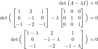
and our goal is to compute the eigenvectors and eigenvalues of this matrix. First, we need to compute the eigenvalues. The eigenvalues are given as the roots of the characteristic polynomial:
(7) 
We can compute the determinant by using the coefficients from the third column. We do that since the computations will simplify due to the zero in the position ![]() . The determinant is given by
. The determinant is given by
(8) 
That is, the characteristic polynomial is
(9) ![]()
Obviously, the eigenvalues are
(10) ![]()
Now, let us compute the corresponding eigenvectors.
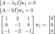
First, we compute the eigenvector ![]() by solving the following system of equations
by solving the following system of equations
(11) 
Let the components of the vector ![]() be given by
be given by
(12) 
Then the system of equations (11) can be written like this
(13) 
We can expand this system of equations like this
(14) 
We want to solve this system by using the Gaussian elimination. First, we multiply the first equation by ![]() and we add the result to the second equation. Then we add the first equation to the third equation. As a result, we obtain
and we add the result to the second equation. Then we add the first equation to the third equation. As a result, we obtain
(15) 
From the second equation, we obtain
(16) ![]()
By substituting this equation into the first equation of (15), we obtain
(17) ![]()
Obviously, the original system of equations has an infinite number of solutions. However, from (16) and (17), we can observe that the solutions are actually parametrized by the following vector
(18) 
where we have complete freedom to select the scalar ![]() . For example, we can select
. For example, we can select ![]() . As the result, we obtain the following eigenvector
. As the result, we obtain the following eigenvector
(19) 
By selecting any other value of ![]() we will also obtain another eigenvector. That is, if we multiply an eigenvector by a constant scalar, the result is also an eigenvector!
we will also obtain another eigenvector. That is, if we multiply an eigenvector by a constant scalar, the result is also an eigenvector!
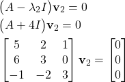
Next, we compute the eigenvector ![]() by solving the following system of equations
by solving the following system of equations
(20) 
By using the parametrization, we obtain
(21) 
The system (20) can be written as
(22) 
or in the expanded version
(23) 
By multiplying the third equation by (-1) and placing it as the first equation, we obtain
(24) 
By multiplying the first equation with (-5) and adding the result to the second equation, and by multiplying the first equation with (-6) and by adding the result to the third equation, we obtain
(25) 
By multiplying the second equation by ![]() and adding the resulting equation to the third equation, we obtain
and adding the resulting equation to the third equation, we obtain
(26) 
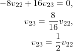
From the second equation, we obtain
(27) 
By substituting this equation in the first equation of (26), we obtain
(28) 
By using (27) and (28), we obtain the parametrized eigenvector
(29) 
By selecting ![]() , we obtain the second eigenvector
, we obtain the second eigenvector
(30) 
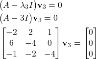
Finally, we compute the eigenvector ![]() by solving the following system of equations
by solving the following system of equations
(31) 
By using the eigenvector
(32) 
The resulting system of equations is
(33) 
By multiplying the third equation by ![]() , and placing as the first equation, we obtain
, and placing as the first equation, we obtain
(34) 
By multiplying the first equation by ![]() and adding the result to the second equation, and by multiplying the first equation by
and adding the result to the second equation, and by multiplying the first equation by ![]() and by adding the result to the third equation, we obtain
and by adding the result to the third equation, we obtain
(35) 
By multiplying the second equation by ![]() and by adding the result to the third equation, we obtain
and by adding the result to the third equation, we obtain
(36) 
From the second equation, we obtain
(37) 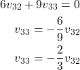
By substituting this result in the first equation of (36), we obtain
(38) 
Consequently, the parametrized vector is
(39) 
By selecting ![]() , we obtain the final expression for the third eigenvector
, we obtain the final expression for the third eigenvector ![]()
(40) 