Implementation of the Solution of the Linear Quadratic Regulator (LQR) Control Algorithm in C++ by Using the Eigen Matrix Library. – Fusion of Engineering, Control, Coding, Machine Learning, and Science

In this control engineering, control theory, computer science, and scientific computing tutorial we explain how to implement a Linear Quadratic Regulator (LQR) control algorithm in C++ from scratch by using the Eigen matrix library. To implement the algorithm, we use the Newton method for solving the underlying Riccati equation. You will learn how to write a C++ class that will in a disciplined and object-oriented manner implement the solution of the LQR control algorithm. Also, you will learn how to write a driver code for using this class. The LQR control algorithm is one of the most popular optimal control algorithms. Consequently, it is very important to know how to properly implement this algorithm in C++. The YouTube tutorial accompanying this website tutorial is given below. The GitHub page with all the code files is given here.

Linear Quadratic Optimal Control Formulation and Riccati Equation

Consider a linear state-space model

(1) $\begin{align*}\dot{\mathbf{x}}=A\mathbf{x}+B\mathbf{u} \\\mathbf{y}=C\mathbf{x}\end{align*}$

where $A\in \mathbb{R}^{n\times n}$ , $B\in \mathbb{R}^{n\times m}$ , and $C\in \mathbb{R}^{r\times n}$ are the system matrices, $\mathbf{x}\in \mathbb{R}^{n}$ is the state vector, and $\mathbf{y}\in \mathbb{R}^{r}$ is the output vector. The linear quadratic optimal control problem, also known as the Linear Quadratic Regulator (LQR) problem, is to determine a state feedback control matrix $K\in \mathbb{R}^{m\times n}$ and the state-feedback control law

(2) $\begin{align*}\mathbf{u}=-K\mathbf{x}\end{align*}$

That will optimize the following cost function

(3) $\begin{align*}\min_{\mathbf{u}} \int_{t=0}^{\infty} \Big( \mathbf{x}^{T}Q\mathbf{x}+ \mathbf{u}^{T}R\mathbf{u}+2\mathbf{x}^{T}S\mathbf{u} \Big)\text{dt}\end{align*}$

where

$Q\in \mathbb{R}^{n\times n}$ is the symmetric positive definite weight matrix that penalizes the speed of the response.
$R\in \mathbb{R}^{m\times m}$ is the symmetric positive definite weight matrix that penalizes the control inputs. That is, it penalizes the control energy.
$S\in \mathbb{R}^{n\times m}$ is the mixed input-state weight matrix.

The solution to the LQR optimization problem, that is the gain matrix $K$ is found by first solving the associated Riccati equation

(4) $\begin{align*}Q+A^{T}X+XA-(B^{T}X+S^{T})^{T}R^{-1}(B^{T}X+S^{T})=0\end{align*}$

where $X\in \mathbb{R}^{n}$ is the solution of the Riccati equation that we want to find. Once the solution $X$ is found, the LQR control gain matrix is determined by

(5) $\begin{align*}K=R^{-1}(B^{T}X+S^{T})\end{align*}$

By applying the computed LQR control law (2) to the system (1), we obtain the closed-loop state equation

(6) $\begin{align*}\dot{\mathbf{x}}=(A-BK)\mathbf{x}\end{align*}$

where the matrix $(A-BK)$ is stable despite the fact that the open-loop matrix $A$ can be unstable. Due to this, the state trajectories $\mathbf{x}$ will asymptotically approach zero. That is, the system is stabilized. Here it should be kept in mind that the LQR is presented for regulator problems. That is, for steering the state trajectory to the equilibrium points. In practice, the state $\mathbf{x}$ is often an error of the feedback control system. That is, the LQR algorithm can easily be modified to be used for designing set-point tracking algorithms. You can learn more about this over here and over here.

Newton Method for Solving the Riccati Equation and for Computing the Solution to the LQR Problem

In the previous section, we learned that in order to compute the solution to the LQR problem, we need to solve the Riccati equation. One of the most elegant methods for solving the Riccati equation is the Newton matrix algorithm. This algorithm is designed for solving nonlinear matrix equations. It transforms the problem of solving the nonlinear Riccati matrix equation into a series of subproblems, where in every subproblem we need to solve the Lyapunov equation. That is, the Newton method iteratively solves the Riccati equation by solving a series of the Lyapunov equations. Here are the two books that thoroughly explain the Newton method for solving the Riccati equation:

“Numerical solution of algebraic Riccati equations”, D. A. Bini, B. Iannazzo, B. Meini, SIAM, (2012). See Section 3.3 in this book.
“The autonomous linear quadratic control problem: theory and numerical solution”, Mehrmann, V. L., Springer, (1991). See page 90 and the corresponding section of this book.

Here is the Netwon method for solving the Riccati equation (taken from Mehrmann’s book and modified):

STEP 1: Compute an initial stabilizing guess of the solution $X_{0}$ . This solution is computed such that the initial closed-loop matrix $\bar{A}_{1}$

(7) $\begin{align*}\bar{A}_{1}& =A-BK_{1}=A-BR^{-1}(B^{T}X_{0}+S^{T}) \\K_{1}& =R^{-1}(B^{T}X_{0}+S^{T})\end{align*}$

is a stable matrix. Here, $K_{1}$ is an initial LQR gain matrix. We explain later on how to compute the initial stabilizing guess $X_{0}$ .

STEP 2: For $k=1,2,\ldots$ , and until convergence, compute the solution $X_{k}$ as follows. First compute the LQR gain at the step $k$ , that is compute $K_{k}$ by using $X_{k-1}$ computed from the previous step $k-1$ :

(8) $\begin{align*}K_{k}=R^{-1}(B^{T}X_{k-1}+S^{T})\end{align*}$

Then, compute the closed-loop matrix $\bar{A}_{k}$ as follows

(9) $\begin{align*}\bar{A}_{k}=A-BK_{k}\end{align*}$

Finally, compute $X_{k}$ by solving the following Lyapunov equation

(10) $\begin{align*}\bar{A}_{k}^{T}X_{k}+X_{k}\bar{A}_{k}=-Q-K_{k}^{T}RK_{k}+SK_{k}+K_{k}^{T}S^{T}\end{align*}$

That is, from the above-presented algorithm we can see that the solution can be computed by solving a series of the Lyapunov equations (10). Before we explain how to solve the Lyapunov equation, we need to explain how to compute the initial stabilizing guess of the solution in step 1. That is, it is very important to initialize this algorithm with a stabilizing solution. This is done in order to guarantee proper convergence of the algorithm to the stabilizing solution.

Method for Computing the Initial Stabilizing Solution

Here, we use an approach that is based on the approach presented in Section 3.3, on page 95 of

“Numerical solution of algebraic Riccati equations”, D. A. Bini, B. Iannazzo, B. Meini, SIAM, (2012). See Section 3.3 in this book.

First, we compute

(11) $\begin{align*}A_{\text{new}}=A-BR^{-1}S^{T},\;\; B_{\text{new}}=BR^{-1}B^{T}\end{align*}$

Then, we compute the eigenvalues of the matrix $A_{\text{new}}$ . Let the real parts of these eigenvalues be denoted by $\lambda_{re,1},\lambda_{re,2},\ldots,\lambda_{re,n}$ (we have $n$ eigenvalues since the matrix $A_{\text{new}}$ is n-dimensional). Then, we compute the parameter $\alpha$

(12) $\begin{align*}\alpha = -1\cdot\min_{\lambda_{re}} \{ \lambda_{re,1},\lambda_{re,2},\ldots, \lambda_{re,n} \}\end{align*}$

That is, $\alpha$ is equal to the minimal value of the real part of the eigenvalues. Then, we define the parameter $\beta$ as

(13) $\begin{align*}\beta=\text{max}(0,\alpha)+\varepsilon\end{align*}$

where $\varepsilon$ is a small number selected by the user. In our case, we are using $\varepsilon=0.02$ . Then, for such computed $\beta$ , we construct the matrix

(14) $\begin{align*}A_{\beta}=A_{\text{new}}+\beta I_{n} \end{align*}$

where $I_{n}$ is $n$ -dimensional identity matrix. Next, we compute the matrix $Z$ by solving this Lyapunov equation

(15) $\begin{align*}A_{\beta}Z+ZA_{\beta}^{T}=2B_{\text{new}}B_{\text{new}}^{T}\end{align*}$

Then, after solving this Lyapunov equation, we compute the initial guess $X_{0}$ of the solution of the Riccati equation as follows:

(16) $\begin{align*}X_{0}=B_{\text{new}}^{T}Z^{-1}\end{align*}$

Under the standard assumption, it is guaranteed that such a solution will stabilize the initial closed-loop matrix $\bar{A}_{1}$ defined in (7). Here again, we see that in order to compute the initial guess of the solution, we need to solve the Lyapunov equation. In our next section, we explain how to solve the Lyapunov equation.

Solve the Lyapunov Equation

From the previous two sections, we learned that we need to solve the Lyapunov equation in order to compute the initial guess and in order to compute the solution of the Lyapunov equation. There are a number of methods for solving the Lyapunov equation. In our previous tutorial, which can be found here, we explained how to solve the Lyapunov equation by using the Kronecker operator approach and matrix vectorization. This approach might not be the most efficient approach from the computational perspective and memory consumption perspective. There are more efficient approaches. However, due to its simplicity, we will use this approach. Here, we will only briefly summarize this approach, and the interested reader is advised to read the above-mentioned tutorial. For generality, let us consider this Lyapunov equation (you can easily change the matrices in order to apply this method to the Lyapunov equations introduced in the previous two sections):

(17) $\begin{align*}M^{T}P+PM=W\end{align*}$

where $M$ is the known coefficient matrix, $W$ is the known right-hand side, and $P$ is the solution that we want to find. By vectorizing the last matrix equation, we obtain (see this tutorial)

(18) $\begin{align*}\Big( I\otimes M^{T}+M^{T}\otimes I\Big) \text{vec}(P)=\text{vec}(W)\end{align*}$

here $\Big( I\otimes M^{T}+M^{T}\otimes I \Big)$ is a matrix, $\text{vec}(P)$ is a vector, and $\text{vec}(W)$ is a vector. The notation $\otimes$ is the standard notation for the Kronecker product, and $\text{vec}(\cdot)$ is the vectorization operator that creates a vector out of a matrix by stacking the columns of the matrix column-wise. The system (18) is a linear system of equations that can easily be solved to compute the vector $\text{vec}(P)$ . Once we compute this vector, we can de-vectorize this equation to compute the matrix $P$ . That is it, simple as that.

Test Case Example

To test the presented LQR solution method, we consider the following test example. We consider a mass-spring damper system as a test case for the model predictive controller. The state-space model of this system is derived in our previous tutorial which can be found here. The model is shown in the figure below.

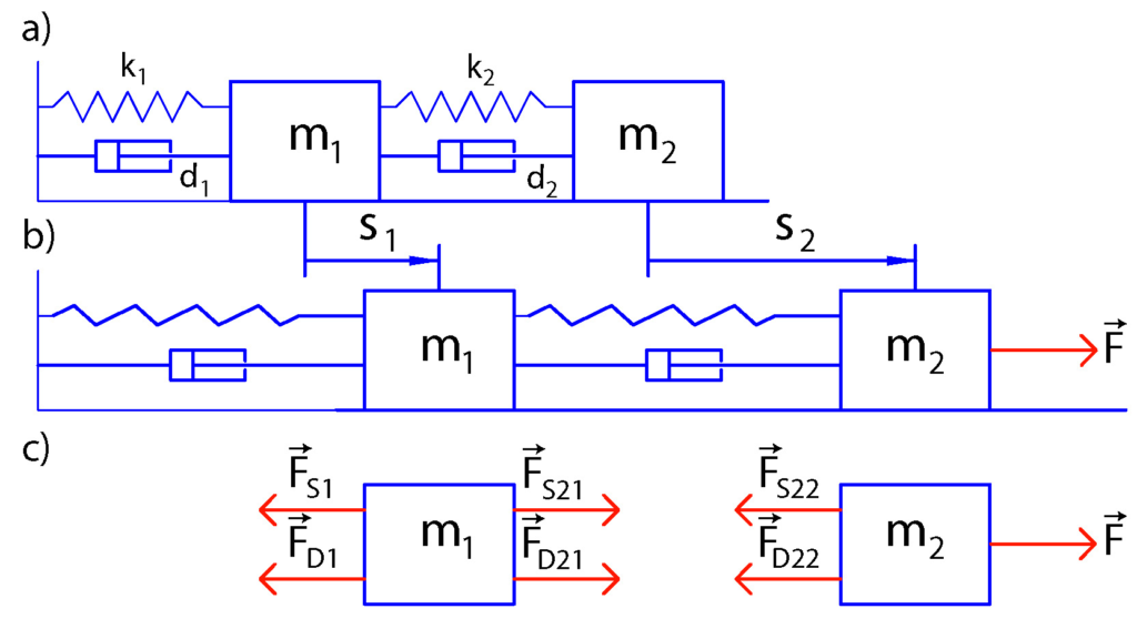
The state-space model has the following form:

(19) $\begin{align*}\underbrace{\begin{bmatrix}\dot{x}_{1} \\ \dot{x}_{2} \\ \dot{x}_{3} \\ \dot{x}_{4}\end{bmatrix}}_{\dot{\mathbf{x}}}= \underbrace{\begin{bmatrix}0 & 1 & 0 & 0 \\ -\frac{k_{1}+k_{2}}{m_{1}} & -\frac{d_{1}+d_{2}}{m_{1}} & \frac{k_{2}}{m_{1}} & \frac{d_{2}}{m_{1}} \\0 & 0 & 0 & 1 \\ \frac{k_{2}}{m_{2}} & \frac{d_{2}}{m_{2}} & -\frac{k_{2}}{m_{2}} & -\frac{d_{2}}{m_{2}} \end{bmatrix}}_{A_{c}} \underbrace{\begin{bmatrix}x_{1} \\ x_{2} \\ x_{3} \\ x_{4}\end{bmatrix}}_{\mathbf{x}}+\underbrace{\begin{bmatrix} 0 \\ 0 \\ 0 \\ \frac{1}{m_{2}} \end{bmatrix}}_{B_{c}}\underbrace{F}_{\mathbf{u}} \end{align*}$

(20) $\begin{align*}\mathbf{y}=\underbrace{\begin{bmatrix}1 & 0 & 0 & 0\end{bmatrix}}_{C}\mathbf{x}\end{align*}$

The next step is to transform the state-space model (19)-(20) in the discrete-time domain. Due to its simplicity and good stability properties, we use the Backward Euler method to perform the discretization. This method approximates the state derivative as follows

(21) $\begin{align*}\frac{\mathbf{x}_{k}-\mathbf{x}_{k-1}}{h}=A_{c}\mathbf{x}_{k}+B_{c}\mathbf{u}_{k-1}\end{align*}$

where $h$ is the discretization constant. For simplicity, we assumed that the discrete-time index of the input is $k-1$ . We can also assume that the discrete-time index of input is $k$ if we want. However, then, when simulating the system dynamics we will start from $k=1$ . From the last equation, we have

(22) $\begin{align*}\mathbf{x}_{k}=A\mathbf{x}_{k-1}+B \mathbf{u}_{k-1} \end{align*}$

where $A=(I-hA_{c})^{-1}$ and $B=hAB_{c}$ . On the other hand, the output equation remains unchanged

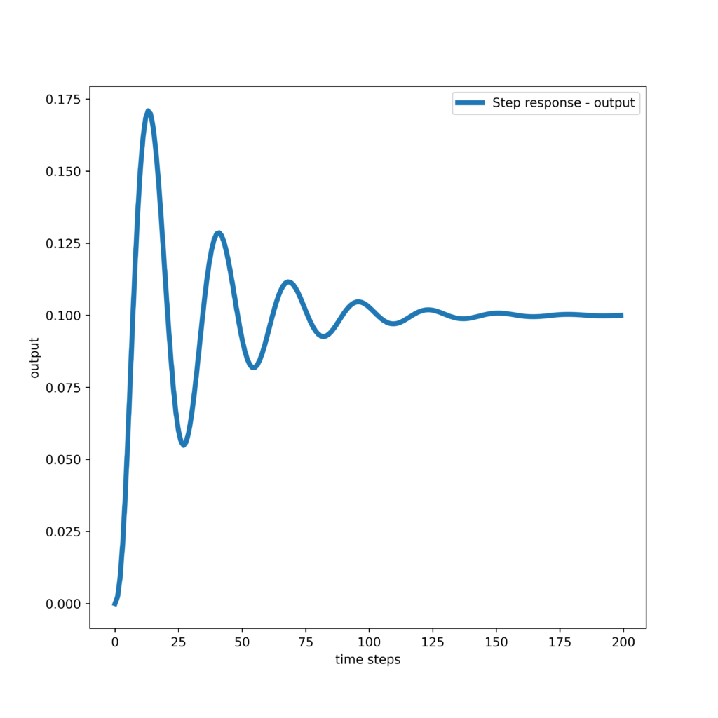
(23) $\begin{align*}\mathbf{y}_{k}=C\mathbf{x}_{k}\end{align*}$

The step response of the system is shown below (the codes are given in the first tutorial part).

C++ Implementation of the Newton Method For Solving the Riccati Equation and the LQR Optimal Control Problem

The GitHub page with all the code files is given here. The codes presented in this section are thoroughly explained in the YouTube video tutorial given at the top of this webpage. Here, for brevity of this tutorial, we will just present the code. The class header file for solving the LQR problem is given below.

/*
Linear Quadratic Regulator (LQR) (Optimal) Controller implementation in C++
Author:Aleksandar Haber 
Date: September 2023 

We implemented a LQR control algorithm in C++ by using the Eigen C++ Matrix library 
The description of the LQR algorithm is given in this tutorial:

This is the header file of the LQR controller class

LICENSE: THIS CODE CAN BE USED FREE OF CHARGE ONLY FOR ACADEMIC AND EDUCATIONAL PURPOSES.
THAT IS, IT CAN BE USED FREE OF CHARGE ONLY IF THE PURPOSE IS NON-COMMERCIAL AND IF THE PURPOSE
IS NOT TO MAKE PROFIT OR EARN MONEY BY USING THIS CODE. 

IF YOU WANT TO USE THIS CODE IN THE COMMERCIAL SETTING, THAT IS, IF YOU WORK FOR A COMPANY OR IF YOU ARE INDEPENDENT
CONSULTANT AND IF YOU WANT TO USE THIS CODE, THEN WITHOUT MY PERMISSION AND WITHOUT PAYING THE PROPER FEE, YOU ARE NOT ALLOWED
TO USE THIS CODE. YOU CAN CONTACT ME AT 

ml.mecheng@gmail.com

TO INFORM YOURSELF ABOUT THE LICENSE OPTIONS AND FEES FOR USING THIS CODE.

*/
#ifndef LQRCONTROLLER_H
#define LQRCONTROLLER_H

#include<string>
#include<Eigen/Dense>
using namespace Eigen;
using namespace std;


class LQRController{
    public:
        // default constructor - edit this later
        LQRController();

        /* 
        This constructor will initialize all the private variables, 
        and precompute some constants
        */
        // Input arguments"
        // Ainput, Binput - A and B system matrices 
        // Qinput - state weighting matrix
        // Rinput - control input weighting matrix
        // Sinput - state-input mixed weighting matrix
                
        LQRController(MatrixXd Ainput, MatrixXd Binput, 
                       MatrixXd Qinput, MatrixXd Rinput,MatrixXd Sinput);
        
                /*
        This function computes the initial guess of the solution of the Riccati equation
        by using the method explained in Section 3.3, page 95 of 
        D. A. Bini, B. Iannazzo, B. Meini - 
        "Numerical solution of algebraic Riccati equations", SIAM, (2012)
        NOTE: The initial guess of the solution should be a stabilizing matrix
        That is, the matrix A-B*K0 is a stable matrix, where K0 is the initial gain computed
        on the basis of the initial guess X0 of the solution of the Riccati equation.
        This function will compute X0.

        Input argument: initialGuessMatrix - this is a reference to the matrix that is used to store 
        the initial guess

        */

        void ComputeInitialGuess(MatrixXd &initialGuessMatrix);

        /*
        This function solves the Lyapunov equation by using the vectorization and Kronecker operator method 
        Am^{T}*SolutionMatrix+SolutionMatrix*A=Rm

        Input arguments:

            Am - input matrix A
            Rm - right hand size matrix Rm
            SolutionMatrix - the solution matrix, it is passed as a reference, that is the solution is 
            stored in this matrix 
            residual - this is the residual to track the accuracy, it is passed as a reference, that is,
            the computed residual is stored in this variable
            The residual is computed as the Frobenius norm of the residual matrix
            Am^{T}*SolutionMatrix+SolutionMatrix*A-Rm
        */
        void SolveLyapunovEquation(const MatrixXd &Am, const MatrixXd &  Rm, MatrixXd &SolutionMatrix, double &residual);
        
        // this function computes the solution by using the Newton algorithm
        void ComputeSolution(int numberIterations, double tolerance);

        /*
            This function is used to simulate the closed loop system
            it will columns of the private member matrix simulatedStateTrajectory
            Input arguments: 
            - x0 - initial condition
            - simulationTimeSteps - total number of simulation time steps
            - h - discretization time step
        */
        void SimulateSystem(MatrixXd x0,int simulationTimeSteps, double h);


        /*
         this function is used to save the variables as "csv" files
         adjust this function as you wish later on
         KFile - name of the file used to store the computed LQR gain matrix K
         AclFile  - name of the file used to store the closed loop matrix
         solutionRiccatiFile  - name of the file used to store the solution of the Riccati equation
         simulatedStateTrajectoryFile  - name of the file used to store the closed loop state trajectory
        */
        void SaveData(string KFile,string AclFile,string solutionRiccatiFile,string simulatedStateTrajectoryFile) const;


    private:

    // MatrixXd is an Eigen typdef for Matrix<double, Dynamic, Dynamic>
	    MatrixXd A,B; // system matrices
        MatrixXd Q,R,S;   // weighting matrices
	   
        MatrixXd K; // LQR control gain matrix 
        MatrixXd Acl; // LQR closed-loop matrix Acl=A-B*K
        MatrixXd solutionRiccati; // solution of the Riccati equation
        MatrixXd In; // identity matrix for computations
        MatrixXd simulatedStateTrajectory; // simulated state trajectory of the closed-loop state-space model

        unsigned int n; // state dimension 
        unsigned int m; // input dimension
      
    
};

#endif

The class implementation file is given below.

/*
Linear Quadratic Regulator (LQR) (Optimal) Controller implementation in C++
Author:Aleksandar Haber 
Date: September 2023 

We implemented a LQR control algorithm in C++ by using the Eigen C++ Matrix library 
The description of the LQR algorithm is given in this tutorial:

This is the implementation file of the LQR controller class

LICENSE: THIS CODE CAN BE USED FREE OF CHARGE ONLY FOR ACADEMIC AND EDUCATIONAL PURPOSES.
THAT IS, IT CAN BE USED FREE OF CHARGE ONLY IF THE PURPOSE IS NON-COMMERCIAL AND IF THE PURPOSE
IS NOT TO MAKE PROFIT OR EARN MONEY BY USING THIS CODE. 

IF YOU WANT TO USE THIS CODE IN THE COMMERCIAL SETTING, THAT IS, IF YOU WORK FOR A COMPANY OR IF YOU ARE INDEPENDENT
CONSULTANT AND IF YOU WANT TO USE THIS CODE, THEN WITHOUT MY PERMISSION AND WITHOUT PAYING THE PROPER FEE, YOU ARE NOT ALLOWED
TO USE THIS CODE. YOU CAN CONTACT ME AT 

ml.mecheng@gmail.com

TO INFORM YOURSELF ABOUT THE LICENSE OPTIONS AND FEES FOR USING THIS CODE.

*/
// C++ includes
#include <iostream>
#include<tuple>
#include<string>
#include<fstream>
#include<vector>
// Eigen header files
#include<Eigen/Dense>
#include <unsupported/Eigen/KroneckerProduct>
#include <Eigen/Eigenvalues> 
// LQR controller header file
#include "LQRController.h"


       /* 
        This constructor will initialize all the private variables, 
        and precompute some constants and matrices
        */
        // Input arguments"
        // Ainput, Binput - A and B system matrices 
        // Qinput - state weighting matrix
        // Rinput - control input weighting matrix
        // Sinput - state-input mixed weighting matrix
                
LQRController::LQRController(MatrixXd Ainput, MatrixXd Binput, 
                       MatrixXd Qinput, MatrixXd Rinput,MatrixXd Sinput)
{
    A=Ainput; B=Binput; Q=Qinput; R=Rinput; S=Sinput;
    n=A.rows(); m=B.cols();


    // create an empty LQR gain matrix
    K.resize(m,n); K.setZero();
    // create an empty closed-loop matrix Acl=A-B*K
    Acl.resize(n,n); Acl.setZero();
    // create an empty matrix for storing the solution of the Riccati equation
    solutionRiccati.resize(n,n);
    solutionRiccati.setZero();
    // identity matrix for computations
    In= MatrixXd::Identity(n,n);
    
    // simulatedStateTrajectory - this private matrix is initialized and resized by the function SimulateSystem()
    // this matrix is the simulated closed-loop state trajectory 
    // this state trajectory is again resized by the function SimulateSystem()
    
    
}

/*
This function computes the initial guess of the solution of the Riccati equation
by using the method explained in Section 3.3, page 95 of 
D. A. Bini, B. Iannazzo, B. Meini - 
"Numerical solution of algebraic Riccati equations", SIAM, (2012)
NOTE: The initial guess of the solution should be a stabilizing matrix
That is, the matrix A-B*K0 is a stable matrix, where K0 is the initial gain computed
on the basis of the initial guess X0 of the solution of the Riccati equation.
This function will compute X0.

Input argument: initialGuessMatrix - this is a reference to the matrix that is used to store 
the initial guess

*/

void LQRController::ComputeInitialGuess(MatrixXd &initialGuessMatrix)
{
    
    // here, we have to introduce new matrices in order to fit everything 
    // in the computational framework explained in the book
    MatrixXd Anew;
    MatrixXd Bnew;
    Anew=A-B*(R.inverse())*(S.transpose());
    Bnew=B*(R.inverse())*(B.transpose());
    
    // compute the eigenvalues of the open-loop matrix
    EigenSolver<MatrixXd> eigenValueSolver(Anew);
    // used to store the current eigenvalue
    complex<double> lambda; 
    // beta parameter from the book
    double bParam=0;
    // we store the real parts of the eigenvalues in this vector
    vector <double> realPartEigenValues;
    // extract the real parts of the eigenvalues and store them in the vector
    for (int i=0; i<n; i++)
    {
        lambda= eigenValueSolver.eigenvalues()[i];
        realPartEigenValues.push_back(lambda.real());
    }
    // compute the bParam
    bParam=(*min_element(realPartEigenValues.begin(), realPartEigenValues.end()));
    //cout<<bParam;
    bParam=(-1)*bParam;
    // be carefull about selecting this constant 0.02, you might need to change it if the convergence 
    // is not fast, 
    bParam=max(bParam,0.0)+0.02;
    // Abar is A+beta*I matrix from the equation 3.14 in the book
    MatrixXd Abar;
    // note that we need to transpose, since our Lyapunov solver is written like this
    // A^{T}X+XA=RHS
    // in the book, it is 
    // AX+XA^{T}=RHS 
    Abar=(bParam*In+Anew).transpose();
    // right-hand side of the equation 3.14 from the book
    MatrixXd RHS;
    RHS=2*Bnew*(Bnew.transpose());
    // solve the Lyapunov equation
    MatrixXd solutionLyapunov;
    solutionLyapunov.resize(n, n); 
    solutionLyapunov.setZero();
    // this residual is filled by the solution residual computed by the Lyapunov solver
    double residualLyap=10e10;
    // call the Lyapunov solver
    SolveLyapunovEquation(Abar, RHS, solutionLyapunov, residualLyap);
    // compute the initial guess matrix by using the equation from the book
    initialGuessMatrix=(Bnew.transpose())*(solutionLyapunov.inverse());
    // ensure that this solution is symmetric - this is a pure heuristic...
    initialGuessMatrix=0.5*(initialGuessMatrix+initialGuessMatrix.transpose());
    //cout<<endl<<"Initial guess of the solution:"<<endl;
    //cout<<endl<<initialGuessMatrix<<endl;
}

/*
This function solves the Lyapunov equation by using the vectorization and Kronecker operator method 
Am^{T}*SolutionMatrix+SolutionMatrix*A=Rm

Input arguments:

    Am - input matrix A
    Rm - right hand size matrix Rm
    SolutionMatrix - the solution matrix, it is passed as a reference, that is the solution is 
    stored in this matrix 
    residual - this is the residual to track the accuracy, it is passed as a reference, that is,
    the computed residual is stored in this variable
    The residual is computed as the Frobenius norm of the residual matrix
    Am^{T}*SolutionMatrix+SolutionMatrix*A-Rm
*/
void LQRController::SolveLyapunovEquation(const MatrixXd &Am, const MatrixXd &  Rm, MatrixXd &SolutionMatrix, double &residual)
{
    // this is the left hand side after we vectorize the Lyapunov equation 
    // by using the Kronecker product
    MatrixXd LHSMatrix;
    // cout<<endl<<Rm<<endl;
    LHSMatrix=kroneckerProduct(In,Am.transpose())+kroneckerProduct(Am.transpose(),In);
    // this variable stores the solution as a vector that is later on resized to be a matrix
    MatrixXd solutionLyapunovVector;
    // this is the right-hand side after we vectorize the Lyapunov equation
    MatrixXd RHSVector;
    // vectorize the input right-hand size matrix
    RHSVector=Rm.reshaped(n*n,1);
    // compute the solution by solving a liner system
    // different options for computing the solution
    //solutionLyapunovVector=LHSMatrix.colPivHouseholderQr().solve(RHSVector);
    //solutionLyapunovVector=LHSMatrix.fullPivLu().solve(RHSVector);
    // solutionLyapunovVector=(LHSMatrix.inverse())*RHSVector;
     solutionLyapunovVector=LHSMatrix.completeOrthogonalDecomposition().solve(RHSVector);
    // reshape the solution vector to be the solution matrix
    SolutionMatrix=solutionLyapunovVector.reshaped(n,n);
    // just in case, make sure that the computed solution is symmetric, pure heuristics...
    SolutionMatrix=0.5*(SolutionMatrix+SolutionMatrix.transpose());
    // this is the residual matrix     
    MatrixXd residualMatrix;
    residualMatrix=(Am.transpose())*SolutionMatrix+SolutionMatrix*Am-Rm;
    // compute the residual by using the Frobenious norm
    residual=residualMatrix.squaredNorm();
}

/*
    This function computes the solution of the LQR problem.
    
    input arguments:

    - maxNumberIterations - maximum number of iterations
    - tolerance - relative convergence tolerance, for example, 1e6 


*/

void LQRController::ComputeSolution(int maxNumberIterations, double tolerance)
{
    // this is the initial guess of the solution
    MatrixXd initialGuess;
    initialGuess.resize(n, n); 
    initialGuess.setZero();
    // call the function for computing the initial guess
    ComputeInitialGuess(initialGuess);

    // check if the initial guess is stabilizing
    // this is very important, otherwise, the convergence cannot be guaranteed
    // initial gain matrix K
    MatrixXd initialK;
    // initial closed-loop matrix
    MatrixXd initialAcl;
    initialK=(R.inverse())*((B.transpose())*initialGuess+S.transpose());
    initialAcl=A-B*initialK;
    // here, we need to compute the eigenvalues of the initial closed loop matrix
    // to make sure that the initial solution is stabilizing
    EigenSolver<MatrixXd> eigenValueSolver(initialAcl);
    cout <<endl<< "The eigenvalues of the initial closed-loop matrix are:" << endl << eigenValueSolver.eigenvalues() << endl;
    cout <<"If all the eigenvalues are strictly in the left-half of the complex plane, the solution is stabilizing!"<<endl;

    // this is the private variable for storing the solution of the Riccati equation
    solutionRiccati= initialGuess;
    // in this matrix, we store the solution of the Lyapunov equation in every iteration
    MatrixXd solutionLyapunov;
    solutionLyapunov.resize(n, n); 
    solutionLyapunov.setZero();
    // matrix to store the right-hand side of the Lyapunov equation
    MatrixXd  RHS;
    // temporary matrix 
    MatrixXd  tmpMatrix;
    // this the update matrix that is used to compute the current relative error
    MatrixXd  updateMatrix;
    // this is the residual of the Lyapunov equation - the value is changed by the Lyapunov solver
    double residualLyap=10e10;
    // this variable is updated by the current value of the errorConvergence
    double errorConvergence=10e10;
    // this variable is used to track the current iteration of the while loop
    int currentIteration=0;
    while  (currentIteration<=maxNumberIterations && errorConvergence>=tolerance )
    {
        /* Approach from Mehrmann's book
         see page 90, of 
        Mehrmann, V. L. (Ed.). (1991). The autonomous linear quadratic control problem: theory and numerical solution. 
        Springer.
        */
        tmpMatrix=(B.transpose())*solutionRiccati+S.transpose();
        // LQR gain is the private variable
        K=(R.inverse())*tmpMatrix;
        // closed loop matrix is actually the private variable
        Acl=A-B*K;
        RHS=Q+(K.transpose())*R*K-S*K-(K.transpose())*(S.transpose());
        // Right-hand side of the Lyapunov equation should be with a minus sign...
        RHS=-RHS;
        // solve the Lyapunov equation
        SolveLyapunovEquation(Acl, RHS, solutionLyapunov, residualLyap);
        // this matrix is only used to track the error convergence
        updateMatrix=solutionLyapunov-solutionRiccati;
        // relative error is the ratio of 1-norms of updateLyapunov and solutionRiccati
        errorConvergence = (updateMatrix.cwiseAbs().colwise().sum().maxCoeff())/(solutionRiccati.cwiseAbs().colwise().sum().maxCoeff());
        // update the solution for the next iteration
        solutionRiccati=solutionLyapunov;
        // increment the iteration number
        currentIteration=currentIteration+1;
        //cout<<currentIteration<<endl;
    }
    // diagnostics
    // if we converged
    if (errorConvergence<tolerance)
    {
        cout<<endl<<"Solution computed within prescribed error tolerances!"<<endl;
        cout<<"Converged error: "<<errorConvergence<<endl;
        cout<<"Number of iterations:"<<currentIteration<<endl;
    }
    // if we did not converge
    if (currentIteration>maxNumberIterations)
    {
        cout<<endl<<"Maximum number of maximum iterations exceeded!"<<endl;
        cout<<"However, the current error is not below the error tolerance."<<endl;
        cout<<"Consider incresing the maximum number of iterations or decreasing the tolerances."<<endl;
        cout<<"Current error:"<<errorConvergence<<endl;
    }
   

    // compute the eigenvalues of the final computed closed loop matrix
    EigenSolver<MatrixXd> eigenValueSolver2(Acl);
    cout <<endl<< "The eigenvalues of the final closed-loop matrix: " << endl << eigenValueSolver2.eigenvalues() << endl;
    cout<<endl<<"Computed K matrix: "<<K<<endl;  
}
/*
    This function is used to simulate the closed loop system
    it will columns of the private member matrix simulatedStateTrajectory
    Input arguments: 
    - x0 - initial condition
    - simulationTimeSteps - total number of simulation time steps
    - h - discretization time step
*/
void LQRController::SimulateSystem(MatrixXd x0,int simulationTimeSteps, double h)
{
    simulatedStateTrajectory.resize(n,simulationTimeSteps);simulatedStateTrajectory.setZero();
    simulatedStateTrajectory.col(0)=x0;    

    // this is the discretized closed-loop matrix
    MatrixXd AclDiscrete;
    AclDiscrete=(In-h*Acl).inverse();
    simulatedStateTrajectory.col(0)=x0;

    for (int i=0; i<simulationTimeSteps-1; i++)
    {   
        simulatedStateTrajectory.col(i+1)=AclDiscrete*simulatedStateTrajectory.col(i);
    }
}

/*
         this function is used to save the variables as "csv" files
         adjust this function as you wish later on
         KFile - name of the file used to store the computed LQR gain matrix K
         AclFile  - name of the file used to store the closed loop matrix
         solutionRiccatiFile  - name of the file used to store the solution of the Riccati equation
         simulatedStateTrajectoryFile  - name of the file used to store the closed loop state trajectory
        */
void LQRController::SaveData(string KFile,string AclFile,string solutionRiccatiFile,string simulatedStateTrajectoryFile) const
{
	const static IOFormat CSVFormat(FullPrecision, DontAlignCols, ", ", "\n");
	
	ofstream file1(KFile);
	if (file1.is_open())
	{
		file1 << K.format(CSVFormat);
		
		file1.close();
	}

	ofstream file2(AclFile);
	if (file2.is_open())
	{
		file2 << Acl.format(CSVFormat);
		file2.close();
	}
	
	ofstream file3(solutionRiccatiFile);
	if (file3.is_open())
	{
		file3 << solutionRiccati.format(CSVFormat);
		file3.close();
	}

	ofstream file4(simulatedStateTrajectoryFile);
	if (file4.is_open())
	{
		file4 << simulatedStateTrajectory.format(CSVFormat);
		file4.close();
	}

  
	
}

The driver code is given below.

/*
Linear Quadratic Regulator (LQR) (Optimal) Controller implementation in C++
Author:Aleksandar Haber 
Date: September 2023 

We implemented a LQR control algorithm in C++ by using the Eigen C++ Matrix library 
The description of the LQR algorithm is given in this tutorial:

This is the driver file of the LQR controller class

LICENSE: THIS CODE CAN BE USED FREE OF CHARGE ONLY FOR ACADEMIC AND EDUCATIONAL PURPOSES.
THAT IS, IT CAN BE USED FREE OF CHARGE ONLY IF THE PURPOSE IS NON-COMMERCIAL AND IF THE PURPOSE
IS NOT TO MAKE PROFIT OR EARN MONEY BY USING THIS CODE. 

IF YOU WANT TO USE THIS CODE IN THE COMMERCIAL SETTING, THAT IS, IF YOU WORK FOR A COMPANY OR IF YOU ARE INDEPENDENT
CONSULTANT AND IF YOU WANT TO USE THIS CODE, THEN WITHOUT MY PERMISSION AND WITHOUT PAYING THE PROPER FEE, YOU ARE NOT ALLOWED
TO USE THIS CODE. YOU CAN CONTACT ME AT 

ml.mecheng@gmail.com

TO INFORM YOURSELF ABOUT THE LICENSE OPTIONS AND FEES FOR USING THIS CODE.

*/

#include <iostream>
#include <vector>

#include<Eigen/Dense>
#include <Eigen/Eigenvalues> 

#include "LQRController.h"
#include "LQRController.cpp"

using namespace Eigen;
using namespace std;


int main()
{
// Here we construct a test case. It is a mass-spring-damper system. 

//# masses, spring and damper constants
double m1=2  ; double m2=2   ; double k1=100  ; double k2=200 ; double d1=1  ; double d2=5; 
//# define the continuous-time system matrices and initial condition

    Matrix <double,4,4> Ac {{0, 1, 0, 0},
                            {-(k1+k2)/m1 ,  -(d1+d2)/m1 , k2/m1 , d2/m1},
                            {0 , 0 ,  0 , 1},
                            {k2/m2,  d2/m2, k2/m2, d2/m2}};
    Matrix <double,4,1> Bc {{0},{0},{0},{1/m2}}; 
    Matrix <double,1,4> Cc {{1,0,0,0}};
    
    // initial condition for simulation of the closed loop system
    Matrix <double,4,1> x0 {{5},{-3},{10},{-1}};

    // total number of simulation steps
    int simulationTimeSteps=50;
    // discretization time step 
    double h=0.1;
    // extract the number of rows and columns
    unsigned int n=Ac.rows();
    unsigned int m=Bc.cols();
    
    // construct the weigthing matrices
    // state weighting matrix
    MatrixXd weightMatrixQ;
    weightMatrixQ= 100*MatrixXd::Identity(n,n);

    // input weighting matrix
    MatrixXd weightMatrixR;
    weightMatrixR= 0.01*MatrixXd::Identity(m,m);
    
    // mixed state-input weighting matrix
    MatrixXd weightMatrixS;
    weightMatrixS.resize(n, m); 
    weightMatrixS.setZero();
    int maxIteration=5000;
    double toleranceConvergence=1e-8;
    
    // construct the LQR controller object
    LQRController lqr(Ac, Bc, weightMatrixQ, weightMatrixR,weightMatrixS);
    // compute the solution
    lqr.ComputeSolution(maxIteration,toleranceConvergence);
    // simulate the system
    lqr.SimulateSystem(x0,simulationTimeSteps,h);
    // save the data
    //void SaveData(string KFile,string AclFile,string solutionRiccatiFile,string simulatedStateTrajectoryFile) const;
    lqr.SaveData("computedK.csv","computedAcl.csv","computedSolutionRiccati.csv","computedSimulatedStateTrajectory.csv");

return 0;
}

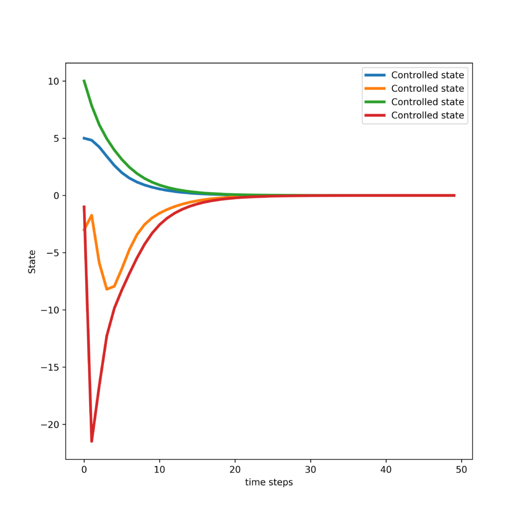
The above-presented driver code will save several CSV files that store the computed LQR matrices and the closed-loop state trajectory. The following Python code will load these matrices and trajectories into the Python workspace and it will plot the trajectories.

# -*- coding: utf-8 -*-
"""
This is the Python file used to visualize the results
and save the graphs

*/
"""

import numpy as np
import matplotlib.pyplot as plt

# Load the matrices and vectors from csv files 
# computed closed loop matrix
AclCpp = np.loadtxt("computedAcl.csv", delimiter=",")
# computed gain matrix
Kcpp = np.loadtxt("computedK.csv", delimiter=",")
# state trajectory
stateCpp= np.loadtxt("computedSimulatedStateTrajectory.csv", delimiter=",")
# solution Riccati
riccatiCpp= np.loadtxt("computedSolutionRiccati.csv", delimiter=",")

# plot the results
plt.figure(figsize=(8,8))
plt.plot(stateCpp.transpose(),linewidth=3, label='Controlled state')
plt.xlabel('time steps')
plt.ylabel('State')
plt.legend()
plt.savefig('controlledState.png',dpi=600)
plt.show()

The following graphs showing the closed-loop state trajectories is generated.

The Python code presented below computes the solution to the LQR control problem by using the Python Control System Toolbox. This code is used to compare the C++ implementation that we developed with the Python implementation.

"""
Linear Quadratic Regulator (LQR) in Python
This Python LQR code is used for comparison with the C++ code

@author: Aleksandar Haber 
date: 2023

pip install slycot   # optional
pip install control

"""

import matplotlib.pyplot as plt
import control as ct
import numpy as np



# masses, spring and damper constants
m1=2  ; m2=2   ; k1=100  ; k2=200 ; d1=1  ; d2=5; 
# define the continuous-time system matrices
A=np.array([[0, 1, 0, 0],
              [-(k1+k2)/m1 ,  -(d1+d2)/m1 , k2/m1 , d2/m1 ],
              [0 , 0 ,  0 , 1], 
              [k2/m2,  d2/m2, k2/m2, d2/m2]])
B=np.array([[0],[0],[0],[1/m2]])
C=np.array([[1, 0, 0, 0]])

D=np.array([[0]])

r=1; m=1 # number of inputs and outputs
n= 4 # state dimension


# define the state-space model
sysStateSpace=ct.ss(A,B,C,D)

#define the initial condition
x0=np.array([[0],[0],[0],[0]])

# print the system
print(sysStateSpace)


##############################################################
# design the LRQ controller
##############################################################


# state weighting matrix
Q=100*np.array([[1,0,0,0],[0,1,0,0],[0,0,1,0],[0,0,0,1]])

# input weighting matrix
R=0.01*np.array([[1]])

# K - gain matrix 
# S - solution of the Riccati equation 
# E - closed-loop eigenvalues 

K, S, E = ct.lqr(sysStateSpace, Q, R)


Acl=A-np.matmul(B,K)

np.linalg.eig(Acl)[0]

Linear Quadratic Optimal Control Formulation and Riccati Equation

Newton Method for Solving the Riccati Equation and for Computing the Solution to the LQR Problem

Method for Computing the Initial Stabilizing Solution

Solve the Lyapunov Equation

Test Case Example

C++ Implementation of the Newton Method For Solving the Riccati Equation and the LQR Optimal Control Problem

admin

You might also like

Definition and Simulation of State-Space Models of Linear Systems in Python by Using Control Systems Library

Control Systems Lecture: Simulation of linear ordinary differential equations using Python and state-space modeling

Pole Placement With Integral Control Action to Eliminate Steady-State Error (State-Space Control Design)