Introduction to Subspace System Identification with Python- System Identification Tutorial – Fusion of Engineering, Control, Coding, Machine Learning, and Science

Introduction

In this post and tutorial, we provide an introduction to Subspace Identification (SI) methods and we develop codes that can be used to effectively estimate Multiple Input -Multiple Output (MIMO) state-space models of dynamical systems. SI methods are effective system identification methods for the estimation of linear MIMO state-space models. There are also a number of extensions of SI methods that can be used for the estimation of nonlinear state-space models. For a relatively broad class of linear state-space problems, subspace identification algorithms perform exceptionally well and outperform most of the algorithms including algorithms based on neural networks.
In contrast to most of the other posts and online lectures, we do not blur the main ideas of the SI algorithm with unnecessary mathematical perplexities and details. Furthermore, to better explain the algorithm, we introduce a model of a physical system and we introduce and provide detailed explanations of Python codes. The YouTube video tutorial accompanying this webpage is given below.

For the impatient, the codes developed and explained in this tutorial can be found here, on my GitHub page.

There are a number of variants of SI methods. In this post, we provide a detailed explanation of a relatively simple SI algorithm that can be used to estimate state-space models of dynamical systems by performing a few relatively simple numerical steps. The main advantage of SI algorithms is that they do not rely upon iterative optimization methods. Instead, they compute estimates of state-space matrices using a least-squares method and using numerical linear algebra methods and algorithms, such as the Singular Value Decomposition (SVD) algorithm, QR decomposition, LU decomposition, etc. The variant of the algorithm that I am going to explain is summarized in this paper (you can cite the paper below if you want to cite this post in your work)

Haber, Aleksandar. “Subspace identification of temperature dynamics.” arXiv preprint arXiv:1908.02379 (2019).
Haber, A., Pecora, F., Chowdhury, M. U., & Summerville, M. (2019, October). Identification of temperature dynamics using subspace and machine learning techniques. In Dynamic Systems and Control Conference (Vol. 59155, p. V002T24A003). American Society of Mechanical Engineers.

We start our discussion with an explanation of the class of models that we want to estimate. We consider a linear state-space model having the following form

(1) $\begin{align*}& \mathbf{x}_{k+1}=A\mathbf{x}_{k}+B\mathbf{u}_{k}+\mathbf{w}_{k} \\ & \mathbf{y}_{k}=C\mathbf{x}_{k}+ \mathbf{n}_{k} \end{align*}$

where $k$ is the discrete time instant, $\mathbf{x}_{k}\in \mathbb{R}^{n}$ is the system state, $n$ is the state order, $\mathbf{u}_{k}\in \mathbb{R}^{m}$ is the control input, $\mathbf{y}_{k}\in \mathbb{R}^{r}$ is the observed output, $\mathbf{w}_{k}\in \mathbb{R}^{n}$ is the process disturbance, $\mathbf{n}_{k}\in \mathbb{R}^{r}$ is the measurement noise, $A\in \mathbb{R}^{n\times n}$ , $B\in \mathbb{R}^{n\times m}$ , and $C\in \mathbb{R}^{r\times n}$ are the system matrices.
The vectors $\mathbf{w}_{k}$ and $\mathbf{n}_{k}$ are usually unknown or only their statistics are known. Under several technical assumptions on the statistics of the vectors $\mathbf{w}_{k}$ and $\mathbf{n}_{k}$ that for simplicity and brevity we do not explain in this post, with the system (1) we can associate another state-space model having the following form

(2) $\begin{align*}& \mathbf{x}_{k+1}=A\mathbf{x}_{k}+B\mathbf{u}_{k}+K\mathbf{e}_{k} \\& \mathbf{y}_{k}=C\mathbf{x}_{k}+\mathbf{e}_{k}\end{align*}$

where $\mathbf{e}_{k}\in \mathbb{R}^{r}$ and $K\in \mathbb{R}^{n\times r}$ . The state-space model (2) is often referred to as the Kalman innovation state-space model. The vector $\mathbf{e}_{k}$ and the matrix $K$ model the effect of the process disturbance and the measurement noise on the system dynamics and the system output. The identification problem can now be formulated as follows.

From the set of input-output data $\{(\mathbf{y}_{i},\mathbf{u}_{i})| i=0,1,2,\ldots, N\}$ estimate the model order $n$ and the system matrices $A, B, C$ and $K$ of the state-space model (2).

It should be emphasized that once the matrices $A, B$ , and $C$ are estimated, we can disregard the matrix $K$ if we want to work with the model (1).

Before we start with the explanation of the SI algorithm, we first introduce a model and codes that are used for the simulation of its response.

Test Model – System of Two Objects Connected by Springs and Dampers

Mass-spring systems are often used as models of a number of physical systems. For example, a car suspension system can effectively be modeled by a mass-spring-damper system. Also, electrical circuits, composed of resistors, inductors, and capacitors (RLC) circuits, have mechanical equivalents that can be physically realized using objects with different masses, springs, and dampers. For these reasons, we focus on mathematical models of mass-spring-damper systems.

The sketch of the system is shown in Fig.1(a) below. The system consists of two objects of the masses $m_{1}$ and $m_{2}$ connected by springs and dampers. In addition, the object 1 is attached to the wall by a spring and a damper. Figure 2(b) shows the situation when the force $\vec{F}$ is acting on the second object. The displacements of the objects $1$ and $2$ from their equilibrium positions are denoted by $s_{1}$ and $s_{2}$ , respectively.

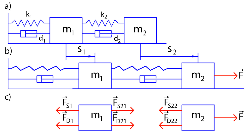Figure 1: (a) The system is composed of two objects connected by springs and dampers. (b) Object displacements when the force $\vec{F}$ is acting on the second body. (c) Free body diagrams of the system.

Figure 1(c) shows the free-body diagrams of the system. The force $\vec{F}_{S1}$ is the force that the spring 1 is exerting on the body 1. The magnitude of this force is given by $|F_{S1}|=|k_{1}s_{1}|$ , where $k_{1}$ is the spring constant. The force $\vec{F}_{D1}$ is the force that the damper 1 is exerting on the body 1. The magnitude of this force is given by $|F_{D1}|=|d_{1}\dot{s}_{1}|$ , where $d_{1}$ is the damper constant and $\dot{s}_{1}$ is the first derivative of the displacement (velocity of the body 1). The force $\vec{F}_{S21}$ is the force that the spring 2 is exerting on the body 1. The magnitude of this force is given by $|F_{S21}|=|k_{2}(s_{2}-s_{1})|$ , where $k_{2}$ is the spring constant. The force $\vec{F}_{D21}$ is the force that the damper 2 is exerting on the body 1. The magnitude of this force is given by $|F_{D21}|=|d_{2}(\dot{s}_{2}-\dot{s}_{1})|$ , where $d_{2}$ is the damper constant.
The force $\vec{F}_{S22}$ is the force that the spring 2 is exerting on the body 2. The force $\vec{F}_{D22}$ is the force that the damper 2 is exerting on the body 2.
We assume that the masses of springs and dampers are much smaller than the masses of the objects and consequently, they can be neglected. Consequently, we have $\vec{F}_{S21}=-\vec{F}_{S22}$ and $\vec{F}_{D21}=-\vec{F}_{D22}$ .

The next step is to apply Newton’s second law:

(3) $\begin{align*} m_{1}\ddot{s}_{1} & = F_{S21} + F_{D21}- F_{S1}-F_{D1} \\m_{2}\ddot{s}_{2} & = F- F_{S22} - F_{D22} \end{align*}$

Then, we introduce the state-space variables

(4) $\begin{align*}x_{1}=s_{1},\;\; x_{2}=\dot{s}_{1}, \;\; x_{3}=s_{2},\;\; x_{4}=\dot{s}_{2} \end{align*}$

By substituting the force expressions in (3) and by using (4) we arrive at the state-space model

(5) $\begin{align*}\underbrace{\begin{bmatrix}\dot{x}_{1} \\ \dot{x}_{2} \\ \dot{x}_{3} \\ \dot{x}_{4}\end{bmatrix}}_{\dot{\mathbf{x}}}= \underbrace{\begin{bmatrix}0 & 1 & 0 & 0 \\ -\frac{k_{1}+k_{2}}{m_{1}} & -\frac{d_{1}+d_{2}}{m_{1}} & \frac{k_{2}}{m_{1}} & \frac{d_{2}}{m_{1}} \\0 & 0 & 0 & 1 \\ \frac{k_{2}}{m_{2}} & \frac{d_{2}}{m_{2}} & -\frac{k_{2}}{m_{2}} & -\frac{d_{2}}{m_{2}} \end{bmatrix}}_{A_{c}} \underbrace{\begin{bmatrix}x_{1} \\ x_{2} \\ x_{3} \\ x_{4}\end{bmatrix}}_{\mathbf{x}}+\underbrace{\begin{bmatrix} 0 \\ 0 \\ 0 \\ \frac{1}{m_{2}} \end{bmatrix}}_{B_{c}}\underbrace{F}_{\mathbf{u}} \end{align*}$

We assume that only the position of the first object can be directly observed. This can be achieved using for example, infrared distance sensors. Under this assumption, the output equation has the following form

(6) $\begin{align*}\mathbf{y}=\underbrace{\begin{bmatrix}1 & 0 & 0 & 0\end{bmatrix}}_{C}\mathbf{x}\end{align*}$

The next step is to transform the state-space model (5)-(6) in the discrete-time domain. Due to its simplicity and good stability properties, we use the Backward Euler method to perform the discretization. This method approximates the state derivative as follows

(7) $\begin{align*}\frac{\mathbf{x}_{k}-\mathbf{x}_{k-1}}{h}=A_{c}\mathbf{x}_{k}+B_{c}\mathbf{u}_{k-1}\end{align*}$

where $h$ is the discretization constant. For simplicity, we assumed that the discrete-time index of the input is $k-1$ . We can also assume that the discrete-time index of input is $k$ if we want. However, then, when simulating the system dynamics we will start from $k=1$ . From the last equation, we have

(8) $\begin{align*}\mathbf{x}_{k}=A\mathbf{x}_{k-1}+B \mathbf{u}_{k-1} \end{align*}$

where $A=(I-hA_{c})^{-1}$ and $B=hAB_{c}$ . On the other hand, the output equation remains unchanged

(9) $\begin{align*}\mathbf{y}_{k}=C\mathbf{x}_{k}\end{align*}$

In the sequel, we present a Python code for discretizing the system and computing the system response to the control input signals. This code will be used to generate identification and validation data.

import numpy as np
import matplotlib.pyplot as plt
from numpy.linalg import inv

# define the system parameters

m1=20  ; m2=20   ; k1=1000  ; k2=2000 ; d1=1  ; d2=5; 


# define the continuous-time system matrices
Ac=np.matrix([[0, 1, 0, 0],[-(k1+k2)/m1 ,  -(d1+d2)/m1 , k2/m1 , d2/m1 ], [0 , 0 ,  0 , 1], [k2/m2,  d2/m2, -k2/m2, -d2/m2]])
Bc=np.matrix([[0],[0],[0],[1/m2]])
Cc=np.matrix([[1, 0, 0, 0]])

#define an initial state for simulation
#x0=np.random.rand(2,1)
x0=np.zeros(shape=(4,1))

#define the number of time-samples used for the simulation and the sampling time for the discretization
time=300
sampling=0.05

#define an input sequence for the simulation
#input_seq=np.random.rand(time,1)
input_seq=5*np.ones(time)
#plt.plot(input_sequence)

I=np.identity(Ac.shape[0]) # this is an identity matrix
A=inv(I-sampling*Ac)
B=A*sampling*Bc
C=Cc


# check the eigenvalues
eigen_A=np.linalg.eig(Ac)[0]
eigen_Aid=np.linalg.eig(A)[0]


# the following function simulates the state-space model using the backward Euler method
# the input parameters are:
#    -- Ad,Bd,Cd           - discrete-time system matrices 
#    -- initial_state      - the initial state of the system 
#    -- time_steps         - the total number of simulation time steps 
# this function returns the state sequence and the output sequence
# they are stored in the matrices Xd and Yd respectively
def simulate(Ad,Bd,Cd,initial_state,input_sequence, time_steps):
    Xd=np.zeros(shape=(A.shape[0],time_steps+1))
    Yd=np.zeros(shape=(C.shape[0],time_steps+1))
    
    for i in range(0,time_steps):
       if i==0:
           Xd[:,[i]]=initial_state
           Yd[:,[i]]=C*initial_state
           x=Ad*initial_state+Bd*input_sequence[i]
       else:
           Xd[:,[i]]=x
           Yd[:,[i]]=C*x
           x=Ad*x+Bd*input_sequence[i]
    Xd[:,[-1]]=x
    Yd[:,[-1]]=C*x
    return Xd, Yd
    
state,output=simulate(A,B,C,x0,input_seq, time)    

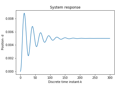
plt.plot(output[0,:])
plt.xlabel('Discrete time instant-k')
plt.ylabel('Position- d')
plt.title('System response')
plt.savefig('step_response1.png')
plt.show()

A few comments are in order. We generate a step control signal. The step response of the system is shown in the figure below. From the step response, we can see that the system is lightly damped. Consequently, due to the complex system poles (in the continuous-time domain), the identification of such a system is far from trivial.

Next, we provide a detailed explanation of the subspace identification method.

Step-by-step Explanation of the Subspace Identification Algorithm

To simplify the derivations and for brevity, we first introduce the following notation.

Let $\mathbf{d}_{k}\in \mathbb{R}^{d_{1}}$ be an arbitrary $d_{1}$ -dimensional vector, where $k$ denotes the discrete-time instant. The notation $\mathbf{d}_{i,j}$ denotes a $(j-i+1)d_{1}$ -dimensional vector defined as follows

(10) $\begin{align*}\mathbf{d}_{i,j}=\begin{bmatrix} \mathbf{d}_{i} \\ \mathbf{d}_{i+1} \\ \vdots \\ \mathbf{d}_{j} \end{bmatrix}\end{align*}$

That is, the vector $\mathbf{d}_{i,j}$ is formed by stacking the vectors $\mathbf{d}_{k}$ on top of each other for an increasing time instant. This procedure is known as the “lifting procedure”.

Using a similar procedure, we define a “data matrix” $D_{i,j}^{(l)}\in \mathbb{R}^{(j-i+1)d_{1}\times (l+1)}$ as follows

(11) $\begin{align*}D_{i,j}^{(l)}=\begin{bmatrix}\mathbf{d}_{i,j} & \mathbf{d}_{i+1,j+1} & ... & \mathbf{d}_{i+l,j+l} \end{bmatrix}\end{align*}$

That is, the matrix $D_{i,j}^{(l)}$ is formed by stacking the vectors $\mathbf{d}_{i+c,j+c}$ and by shifting the time index $c$ . Next, we need to define an operator that extracts rows or columns of a matrix.

Let $X$ be an arbitrary matrix. The notation $X(i:j,:)$ denotes a new matrix that is created from the rows $i, i+1, \ldots, j$ of the matrix $X$ (without row permutations).

Similarly, the notation $X(:,i:j)$ stands for a matrix constructed from the corresponding columns of the matrix $X$ . This notation is inspired by the standard MATLAB notation which is also used in the Python programming language.

Step 1: Estimation of the VARX model or the System Markov Parameters

The abbreviation VARX, stands for Vector Auto-Regressive eXogenous. From the output equation of (2), we can express the innovation vector $\mathbf{e}_{k}$ :

(12) $\begin{align*}\mathbf{e}_{k}=\mathbf{y}_{k}-C\mathbf{x}_{k}\end{align*}$

By substituting this expression in the state equation of the model (2), we obtain the following equation

(13) $\begin{align*}\mathbf{x}_{k+1}& =A\mathbf{x}_{k}+B\mathbf{u}_{k}+K(\mathbf{y}_{k}-C\mathbf{x}_{k}) \\\mathbf{x}_{k+1}& =(A-KC)\mathbf{x}_{k}+B\mathbf{u}_{k}+K\mathbf{y}_{k}\end{align*}$

The last equation can be written compactly as follows

(14) $\begin{align*}\mathbf{x}_{k+1}= \tilde{A}\mathbf{x}_{k}+\tilde{B}\mathbf{z}_{k}\end{align*}$

where

(15) $\begin{align*}\mathbf{z}_{k}=\begin{bmatrix} \mathbf{u}_{k} \\ \mathbf{y}_{k} \end{bmatrix},\;\; \tilde{A}=A-KC,\;\; \tilde{B}=\begin{bmatrix}B & K\end{bmatrix} \end{align*}$

For the development of the SI algorithm, it is important to introduce the parameter $p$ which is referred to as the “past window”. Starting from the time instant $k-p$ , and by performing recursive substitutions of the equation (14), we obtain

(16) $\begin{align*}\mathbf{x}_{k-p+1} & = \tilde{A}\mathbf{x}_{k-p}+\tilde{B}\mathbf{z}_{k-p} \notag \\\mathbf{x}_{k-p+2} & = \tilde{A}\mathbf{x}_{k-p+1}+\tilde{B}\mathbf{z}_{k-p+1}=\tilde{A}^{2}\mathbf{x}_{k-p}+\tilde{A}\tilde{B}\mathbf{z}_{k-p}+\tilde{B}\mathbf{z}_{k-p+1} \notag \\\mathbf{x}_{k-p+3} & = \tilde{A}\mathbf{x}_{k-p+2}+\tilde{B}\mathbf{z}_{k-p+2}=\tilde{A}^{3}\mathbf{x}_{k-p} + \begin{bmatrix}\tilde{A}^{2}\tilde{B} & \tilde{A}\tilde{B} & \tilde{B} \end{bmatrix} \begin{bmatrix}\mathbf{z}_{k-p} \\ \mathbf{z}_{k-p+1} \\ \mathbf{z}_{k-p+2} \end{bmatrix}\end{align*}$

Following this procedure, we obtain

(17) $\begin{align*}\mathbf{x}_{k}=\tilde{A}^{p}\mathbf{x}_{k-p}+\underbrace{\begin{bmatrix}\tilde{A}^{p-1}\tilde{B} & \tilde{A}^{p-2}\tilde{B} & \ldots & \tilde{B} \end{bmatrix}}_{\mathcal{K}_{p-1}} \underbrace{\begin{bmatrix}\mathbf{z}_{k-p} \\ \mathbf{z}_{k-p+1} \\ \vdots \\ \mathbf{z}_{k-1} \end{bmatrix}}_{\mathbf{z}_{k-p,k-1}}\end{align*}$

By multiplying (17) from left by $C$ and by using the output equation(2), we can obtain

(18) $\begin{align*}\mathbf{y}_{k}=C\tilde{A}^{p}\mathbf{x}_{k-p}+\mathcal{M}_{p-1}\mathbf{z}_{k-p,k-1}+\mathbf{e}_{k}\end{align*}$

where

(19) $\begin{align*}\mathcal{M}_{p-1}=C\mathcal{K}_{p-1}=\begin{bmatrix}C\tilde{A}^{p-1}\tilde{B} & C\tilde{A}^{p-2}\tilde{B} & \ldots & C\tilde{B} \end{bmatrix}\end{align*}$

The matrix $\mathcal{M}_{p-1}$ is the matrix of “Markov parameters”. Due to the fact that the matrix $\tilde{A}$ is stable (even if the matrix $A$ is unstable, under some relatively mild assumptions we can determine the matrix $K$ such that the matrix $\tilde{A}$ is stable), we have

(20) $\begin{align*}\tilde{A}^{p}\approx 0\end{align*}$

for sufficiently large $p$ . By substituting (20) in (18), we obtain

(21) $\begin{align*}\mathbf{y}_{k}\approx \mathcal{M}_{p-1}\mathbf{z}_{k-p,k-1}+\mathbf{e}_{k}\end{align*}$

This equation represents VARX model. Namely, the system output at the time instant $k$ depends on the past inputs and outputs contained in the vector $\mathbf{z}_{k-p,k-1}$ . The first step in the SI algorithm is to estimate the Markov parameters of the VARX model. That is, to estimate the matrix $\mathcal{M}_{p-1}$ .

This can be achieved by solving a least-squares problem. Namely, from (21), we can write:

(22) $\begin{align*}&\underbrace{\begin{bmatrix}\mathbf{y}_{p} & \mathbf{y}_{p+1} & \ldots & \mathbf{y}_{p+l}\end{bmatrix}}_{Y_{p,p}^{(l)}} \approx \mathcal{M}_{p-1}\underbrace{\begin{bmatrix} \mathbf{z}_{0,p-1} & \mathbf{z}_{1,p} & \ldots & \mathbf{z}_{l,l+p-1} \end{bmatrix}}_{Z_{0,p-1}^{(l)}}\notag \\ & +\underbrace{\begin{bmatrix} \mathbf{e}_{p} & \mathbf{e}_{p+1} & \ldots & \mathbf{e}_{p+l} \end{bmatrix}}_{E_{p,p}^{(l)}}\end{align*}$

On the basis of the last equation, we can form the least-squares problem

(23) $\begin{align*}\min_{\mathcal{M}_{p-1}} \left\|Y_{p,p}^{(l)}-\mathcal{M}_{p-1} Z_{0,p-1}^{(l)} \right\|_{F}^{2}\end{align*}$

where $\left\| \cdot \right\|_{F}$ is the Frobenius matrix norm. The solution is given by

(24) $\begin{align*} \hat{\mathcal{M}}_{p-1} = Y_{p,p}^{(l)} \big(Z_{0,p-1}^{(l)}\big)^{T} \Big(Z_{0,p-1}^{(l)}\big(Z_{0,p-1}^{(l)} \big)^{T} \Big)^{-1}\end{align*}$

Next, we present the Python code to estimate the Markov parameters.

###############################################################################
# This function estimates the Markov parameters of the state-space model:
# x_{k+1} =  A x_{k} + B u_{k} + Ke(k)
# y_{k}   =  C x_{k} + e(k)
# The function returns the matrix of the Markov parameters of the model
# Input parameters:

# "U" - is the input vector of the form U \in mathbb{R}^{m \times timeSteps}
# "Y" - is the output vector of the form Y \in mathbb{R}^{r \times timeSteps}
# "past" is the past horizon

# Output parameters:
#  The problem beeing solved is
#  min_{M_pm1} || Y_p_p_l -  M_pm1 Z_0_pm1_l ||_{F}^{2}
# " M_pm1" - matrix of the Markov parameters
# "Z_0_pm1_l" - data matrix used to estimate the Markov parameters,
# this is an input parameter for the "estimateModel()" function
# "Y_p_p_l" is the right-hand side 


def estimateMarkovParameters(U,Y,past):
    import numpy as np
    import scipy 
    from scipy import linalg
    
    timeSteps=U.shape[1]
    m=U.shape[0]
    r=Y.shape[0]
    l=timeSteps-past-1
    
    # data matrices for estimating the Markov parameters
    Y_p_p_l=np.zeros(shape=(r,l+1))
    Z_0_pm1_l=np.zeros(shape=((m+r)*past,l+1))  # - returned
    # the estimated matrix that is returned as the output of the function
    M_pm1=np.zeros(shape=(r,(r+m)*past))   # -returned
    
    
    # form the matrices "Y_p_p_l" and "Z_0_pm1_l"
    # iterate through columns
    for j in range(l+1):
        # iterate through rows
        for i in range(past):
            Z_0_pm1_l[i*(m+r):i*(m+r)+m,j]=U[:,i+j]
            Z_0_pm1_l[i*(m+r)+m:i*(m+r)+m+r,j]=Y[:,i+j]
        Y_p_p_l[:,j]=Y[:,j+past]
        # numpy.linalg.lstsq
        #M_pm1=scipy.linalg.lstsq(Z_0_pm1_l.T,Y_p_p_l.T)
        M_pm1=np.matmul(Y_p_p_l,linalg.pinv(Z_0_pm1_l))
    
    return M_pm1, Z_0_pm1_l, Y_p_p_l
###############################################################################
# end of function
###############################################################################

To estimate the Markov parameters, we need to select the past window $p$ . The problem of optimal selection of the past window is an important problem, and we will deal with this problem in our next post.

Step 2: Estimation of the State-Sequence

Once the Markov parameters are estimated, we can proceed with the estimation of the state sequence. The main idea is that if we would know the state sequence $\mathbf{x}_{0},\mathbf{x}_{1}, \ldots, \mathbf{x}_{N}$ , then we would be able to estimate the system matrices $A,B,C$ and $K$ of the state-space model (2) using a simple least-squares method.

Let us write again the equations (17) and (20)

(25) $\begin{align*}\mathbf{x}_{k}=\tilde{A}^{p}\mathbf{x}_{k-p}+\underbrace{\begin{bmatrix}\tilde{A}^{p-1}\tilde{B} & \tilde{A}^{p-2}\tilde{B} & \ldots & \tilde{B} \end{bmatrix}}_{\mathcal{K}_{p-1}} \underbrace{\begin{bmatrix}\mathbf{z}_{k-p} \\ \mathbf{z}_{k-p+1} \\ \vdots \\ \mathbf{z}_{k-1} \end{bmatrix}}_{\mathbf{z}_{k-p,k-1}}\end{align*}$

(26) $\begin{align*}\tilde{A}^{p}\approx 0\end{align*}$

From these two equations, we have

(27) $\begin{align*}\mathbf{x}_{k}\approx \mathcal{K}_{p-1}\mathbf{z}_{k-p,k-1}\end{align*}$

Besides the past window $p$ , another user-selected parameter is defined in the SI algorithm. This parameter is called the future window and is usually denoted by $f$ .

The future window needs to satisfy the following condition $f\le p$ . For a selected value of the future window $f$ , we define the following matrix

(28) $\begin{align*}\mathcal{O}_{f-1}=\begin{bmatrix} C \\ C\tilde{A} \\ C\tilde{A}^{2} \\ \vdots \\ C\tilde{A}^{f-1}\end{bmatrix}\end{align*}$

By multiplying the equation (27) with $\mathcal{O}_{f-1}$ , we obtain

(29) $\begin{align*}& \mathcal{O}_{f-1}\mathbf{x}_{k} \\& \approx \begin{bmatrix} C\tilde{A}^{p-1}B & C\tilde{A}^{p-2}\tilde{B} & C\tilde{A}^{p-3}\tilde{B} &\ldots & \ldots & C\tilde{B}\\ C\tilde{A}^{p}B & C\tilde{A}^{p-1}\tilde{B} & C\tilde{A}^{p-2}\tilde{B} & \ldots & \ldots & C\tilde{A}\tilde{B} \\C\tilde{A}^{p+1}B & C\tilde{A}^{p}\tilde{B} & C\tilde{A}^{p-1}\tilde{B} &\ldots & \ldots & C\tilde{A}^{2}\tilde{B} \\\vdots & \vdots & \vdots & & & \vdots \\ C\tilde{A}^{p+f-2}B & C\tilde{A}^{p+f-3}\tilde{B} & C\tilde{A}^{p+f-4}\tilde{B} & \ldots & \ldots & C\tilde{A}^{f-1}\tilde{B} \end{bmatrix}\mathbf{z}_{k-p,k-1}\end{align*}$

Taking the assumption (20) into account, from (29), we have

(30) $\begin{align*}& \mathcal{O}_{f-1}\mathbf{x}_{k}\approx \\& \underbrace{\begin{bmatrix} C\tilde{A}^{p-1}B & C\tilde{A}^{p-2}\tilde{B} & C\tilde{A}^{p-3}\tilde{B} &\ldots &\ldots & C\tilde{B}\\ 0 & C\tilde{A}^{p-1}\tilde{B} & C\tilde{A}^{p-2}\tilde{B} & \ldots & \ldots & C\tilde{A}\tilde{B} \\0 & 0 & C\tilde{A}^{p-1}\tilde{B} & \ldots & \ldots & C\tilde{A}^{2}\tilde{B} \\\vdots &\vdots & & & \\ 0 & 0 & \ldots 0 & C\tilde{A}^{p-1}\tilde{B} & \ldots & C\tilde{A}^{f-1}\tilde{B} \end{bmatrix}}_{\mathcal{Q}_{p-1}}\mathbf{z}_{k-p,k-1}\end{align*}$

Now, let us analyze the matrix $\mathcal{Q}_{p-1}$ in (30). Its first block row is the matrix $\mathcal{M}_{p-1}$ . Its second block row is the matrix composed of a block zero matrix and the matrix $\mathcal{M}_{p-1}$ in which the last block has been erased, etc. That is, the matrix $\mathcal{Q}_{p-1}$ can be completely reconstructed using the Markov parameter matrix. Let $\hat{\mathcal{Q}}_{p-1}$ denote the matrix constructed on the basis of the estimated matrix $\hat{\mathcal{M}}_{p-1}$ . This matrix is formally defined as follows:

(31) $\begin{align*}\hat{\mathcal{Q}}_{p-1}=\begin{bmatrix}\hat{\mathcal{M}}_{p-1} \\ 0 \; \hat{\mathcal{M}}_{p-1}\big(:,1:(p-1)(r+m)\big) \\ \vdots \\ 0 \ldots \; \; 0 \; \hat{\mathcal{M}}_{p-1}\big(:,1:(p-f+1)(r+m)\big) \end{bmatrix}\end{align*}$

On the basis of the equations (30) and (31), and by iterating the index $k$ from $k=p$ to $k=p+l$ , we obtain

(32) $\begin{align*}\mathcal{O}_{f-1}\underbrace{\begin{bmatrix}\mathbf{x}_{p} & \mathbf{x}_{p+1} & \ldots & \mathbf{x}_{p+l}\end{bmatrix}}_{X_{p,p}^{(l)}}= \hat{\mathcal{Q}}_{p-1}\underbrace{\begin{bmatrix}\mathbf{z}_{0,p-1} & \mathbf{z}_{1,p} & \ldots & \mathbf{z}_{l,p+l-1}\end{bmatrix}}_{Z_{0,p-1}^{(l)}}\end{align*}$

Now, let us analyze the equation (32). We are interested in obtaining an estimate of the matrix $X_{p,p}^{(l)}$ that represents the state sequence. That is, we want to obtain an estimate of the state sequence such that in the later stage we can use this estimate to determine the system matrices. The left-hand side of the equation is completely unknown and the right-hand side is known since we have estimated the matrix $\hat{\mathcal{Q}}_{p-1}$ . If we would know the matrix $\mathcal{O}_{f-1}$ , then we would be able to solve this equation for $X_{p,p}^{(l-1)}$ . However, we do not know this matrix and it seems that our efforts to estimate the model are doomed to fail.

Now, here comes the magic of numerical linear algebra! Under some assumptions, from the equation (32) it follows that we can obtain an estimate of the matrix $X_{p,p}^{(l)}$ by computing a row space of the matrix $\hat{\mathcal{Q}}_{p-1}Z_{0,p-1}^{(l)}$ . The row space can be computed by computing the singular value decompostion (SVD)

(33) $\begin{align*}\hat{\mathcal{Q}}_{p-1}Z_{0,p-1}^{(l)}=U \Sigma V^{T}\end{align*}$

where $U,V$ are orthonormal matrices, and the matrix $\Sigma$ is the matrix of singular values. Let $\hat{n}$ , denote an estimate of the state order (we will explain in the sequel a simple method to estimate the state order, and a more complex method will be explained in our next post). Then, an estimate of the matrix $X_{p,p}^{(l)}$ , denoted by $\hat{X}_{p,p}^{(l)}$ , is computed as follows

(34) $\begin{align*}\hat{X}_{p,p}^{(l-1)}=\Sigma(1:\hat{n},1:\hat{n})^{1/2}V_{T}(1:\hat{n},:)\end{align*}$

where $V_{T}=V^{T}$ and the superscript $1/2$ means that we are taking square roots of the diagonal entries of the matrix $\Sigma(1:\hat{n},1:\hat{n})$ . Once we have estimated the matrix $\hat{X}_{p,p}^{(l)}$ we can obtain the estimate of the state sequence because:

(35) $\begin{align*}\hat{X}_{p,p}^{(l)}=\begin{bmatrix}\hat{\mathbf{x}}_{p} & \hat{\mathbf{x}}_{p+1} & \ldots & \hat{\mathbf{x}}_{p+l} \end{bmatrix}\end{align*}$

Step 3: Estimation of the System Matrices

Now that we have estimated the state sequence, we can estimate the system matrices by forming two least squares problems. Let us write the equation (14) once more over here for clarity

(36) $\begin{align*}\mathbf{x}_{k+1}= \tilde{A}\mathbf{x}_{k}+\tilde{B}\mathbf{z}_{k}\end{align*}$

where

(37) $\begin{align*}\mathbf{z}_{k}=\begin{bmatrix} \mathbf{u}_{k} \\ \mathbf{y}_{k} \end{bmatrix},\;\; \tilde{A}=A-KC,\;\; \tilde{B}=\begin{bmatrix}B & K\end{bmatrix} \end{align*}$

From this equation, we have

(38) $\begin{align*}& \underbrace{\begin{bmatrix}\hat{\mathbf{x}}_{p+1} & \hat{\mathbf{x}}_{p+2} & \ldots & \hat{\mathbf{x}}_{p+l} \end{bmatrix}}_{\hat{X}_{p+1,p+1}^{(l-1)}} \approx \underbrace{\begin{bmatrix} \tilde{A} & \tilde{B} \end{bmatrix}}_{Q}\begin{bmatrix} \hat{\mathbf{x}}_{p} & \hat{\mathbf{x}}_{p+1} & \ldots & \hat{\mathbf{x}}_{p+l-1} \\ \mathbf{z}_{p} & \mathbf{z}_{p+1} & \ldots & \mathbf{z}_{p+l-1} \end{bmatrix} \\& = Q \underbrace{\begin{bmatrix}\hat{X}_{p,p}^{(l-1)} \\ Z_{p,p}^{(l-1)} \end{bmatrix}}_{S} \end{align*}$

Since the matrix $S$ is known, the matrix $Q$ can be estimated by solving

(39) $\begin{align*}\min_{Q} \left\|\hat{X}_{p+1,p+1}^{(l-1)}-Q S \right\|_{F}^{2}\end{align*}$

The solution is given by

(40) $\begin{align*}\hat{Q} = \hat{X}_{p+1,p+1}^{(l-1)} S^{T} \Big(SS^{T} \Big)^{-1}\end{align*}$

Similarly, from the output equation of (2), we have:

(41) $\begin{align*}\underbrace{\begin{bmatrix}\mathbf{y}_{p} & \mathbf{y}_{p+1} & \ldots & \mathbf{y}_{p+l}\end{bmatrix}}_{Y_{p,p}^{(l)}}\approx C \hat{X}_{p,p}^{(l)}\end{align*}$

and the matrix $C$ can be estimated by forming a similar least squares problem

(42) $\begin{align*}\min_{C} \left\| Y_{p,p}^{(l)}-C \hat{X}_{p,p}^{(l)}\right\|_{F}^{2}\end{align*}$

The solution is given by

(43) $\begin{align*}\hat{C} = Y_{p,p}^{(l)} (\hat{X}_{p,p}^{(l)})^{T} \Big(\hat{X}_{p,p}^{(l)}\big(\hat{X}_{p,p}^{(l)} \big)^{T} \Big)^{-1}\end{align*}$

Once these matrices have been estimated, we can obtain the system matrices as follows:

(44) $\begin{align*}& \hat{\tilde{A}}=\hat{Q}(:,1:\hat{n}), \; \hat{B}=\hat{Q}(:,\hat{n}+1:\hat{n}+m), \\ & \; \hat{K}=\hat{Q}(:,\hat{n}+m+1:\hat{n}+m+r),\;\; \hat{A}=\hat{\tilde{A}}+\hat{K}\hat{C} \end{align*}$

where the estimates of the matrices $A,B,C$ , and $K$ are denoted by $\hat{A},\hat{B},\hat{C}$ , and $\hat{K}$ , respectively.

The Python code for estimating the matrices is given below.

###############################################################################
# This function estimates the state-space model:
# x_{k+1} =  A x_{k} + B u_{k} + Ke(k)
# y_{k}   =  C x_{k} + e(k)
# Acl= A - KC
    
# Input parameters:
    
# "U" - is the input matrix of the form U \in mathbb{R}^{m \times timeSteps}
# "Y" - is the output matrix of the form Y \in mathbb{R}^{r \times timeSteps}
# "Markov" - matrix of the Markov parameters returned by the function "estimateMarkovParameters()"
# "Z_0_pm1_l" - data matrix returned by the function "estimateMarkovParameters()"      
# "past" is the past horizon
# "future" is the future horizon
# Condition: "future" <= "past"
# "order_estimate" - state order estimate
    
# Output parameters:
# the matrices: A,Acl,B,K,C
# s_singular - singular values of the matrix used to estimate the state-sequence
# X_p_p_l   - estimated state sequence    
    
    
def estimateModel(U,Y,Markov,Z_0_pm1_l,past,future,order_estimate):
    import numpy as np
    from scipy import linalg
    
    timeSteps=U.shape[1]
    m=U.shape[0]
    r=Y.shape[0]
    l=timeSteps-past-1
    n=order_estimate
    
    Qpm1=np.zeros(shape=(future*r,past*(m+r)))
    for i in range(future):
        Qpm1[i*r:(i+1)*r,i*(m+r):]=Markov[:,:(m+r)*(past-i)]
    
    
    
    # estimate the state sequence
    Qpm1_times_Z_0_pm1_l=np.matmul(Qpm1,Z_0_pm1_l)
    Usvd, s_singular, Vsvd_transpose = np.linalg.svd(Qpm1_times_Z_0_pm1_l, full_matrices=True)
    # estimated state sequence
    X_p_p_l=np.matmul(np.diag(np.sqrt(s_singular[:n])),Vsvd_transpose[:n,:])    
    
    
    X_pp1_pp1_lm1=X_p_p_l[:,1:]
    X_p_p_lm1=X_p_p_l[:,:-1]
    
    # form the matrices Z_p_p_lm1 and Y_p_p_l
    Z_p_p_lm1=np.zeros(shape=(m+r,l))
    Z_p_p_lm1[0:m,0:l]=U[:,past:past+l]
    Z_p_p_lm1[m:m+r,0:l]=Y[:,past:past+l]
    
    Y_p_p_l=np.zeros(shape=(r,l+1))
    Y_p_p_l=Y[:,past:]
        
    S=np.concatenate((X_p_p_lm1,Z_p_p_lm1),axis=0)
    ABK=np.matmul(X_pp1_pp1_lm1,np.linalg.pinv(S))
    
    C=np.matmul(Y_p_p_l,np.linalg.pinv(X_p_p_l))
    Acl=ABK[0:n,0:n]
    B=ABK[0:n,n:n+m]  
    K=ABK[0:n,n+m:n+m+r]  
    A=Acl+np.matmul(K,C)
    
    
    return A,Acl,B,K,C,s_singular,X_p_p_l
###############################################################################
# end of function
###############################################################################

Model estimation in practice

To identify the model and test the model performance, we need to generate two sets of data. The first set of data, referred to as the identification data set is used to identify the model. This data set is generated for a random initial condition and for a random input sequence. Not every input sequence can be used for system identification.

The input sequence needs to satisfy the so-called persistency of the excitation condition. Loosely speaking, the identification sequence needs to be rich enough to excite all the system modes. Usually, a random sequence will satisfy this condition. Besides, the identification data set, we are using another data set. This data set, which is referred to as the validation data set is used to test the estimated model performance. This data set is generated for a random initial condition and for a random input sequence. The validation initial state and the input sequence are generated such that they are statistically independent from the initial state and the input sequence used for the identification.

All the functions used for the identification are stored in the file “functionsSID”. Here we provide a detailed explanation of the driver code. As a numerical example, we use the example introduced at the beginning of this post. We start with an explanation of the code. The following code is used to import the necessary functions and to define the model.

import numpy as np
import matplotlib.pyplot as plt
from numpy.linalg import inv

from functionsSID import estimateMarkovParameters
from functionsSID import estimateModel
from functionsSID import systemSimulate
from functionsSID import estimateInitial
from functionsSID import modelError

###############################################################################
# Define the model

# masses, spring and damper constants
m1=20  ; m2=20   ; k1=1000  ; k2=2000 ; d1=1  ; d2=5; 
# define the continuous-time system matrices
Ac=np.matrix([[0, 1, 0, 0],[-(k1+k2)/m1 ,  -(d1+d2)/m1 , k2/m1 , d2/m1 ], [0 , 0 ,  0 , 1], [k2/m2,  d2/m2, -k2/m2, -d2/m2]])
Bc=np.matrix([[0],[0],[0],[1/m2]])
Cc=np.matrix([[1, 0, 0, 0]])
# end of model definition
###############################################################################

###############################################################################

The following code lines are used to define the identification parameters and to define the identification and validation data sets.

###############################################################################
# parameter definition

r=1; m=1 # number of inputs and outputs
# total number of time samples
time=300
# discretization constant
sampling=0.05

# model discretization
I=np.identity(Ac.shape[0]) # this is an identity matrix
A=inv(I-sampling*Ac)
B=A*sampling*Bc
C=Cc

# check the eigenvalues
eigen_A=np.linalg.eig(Ac)[0]
eigen_Aid=np.linalg.eig(A)[0]

# define an input sequence and initial state for the identification
input_ident=np.random.rand(1,time)
x0_ident=np.random.rand(4,1)

#define an input sequence and initial state for the validation
input_val=np.random.rand(1,time)
x0_val=np.random.rand(4,1)

# simulate the discrete-time system to obtain the input-output data for identification and validation
Y_ident, X_ident=systemSimulate(A,B,C,input_ident,x0_ident)
Y_val, X_val=systemSimulate(A,B,C,input_val,x0_val)

#  end of parameter definition
###############################################################################

A few comments are in order. The code lines 11-14 are used to discretize the model. The code lines 17-18 are used to check the eigenvalues of the models. This is important for detecting possible instabilities. The code lines 21-30 are used to define the identification and validation data sets.

The following code is used to estimate the model and to perform the model validation.

###############################################################################
# model estimation and validation

# estimate the Markov parameters
past_value=10 # this is the past window - p 
Markov,Z, Y_p_p_l =estimateMarkovParameters(input_ident,Y_ident,past_value)

# estimate the system matrices
model_order=3 # this is the model order \hat{n}
Aid,Atilde,Bid,Kid,Cid,s_singular,X_p_p_l = estimateModel(input_ident,Y_ident,Markov,Z,past_value,past_value,model_order)  

plt.plot(s_singular, 'x',markersize=8)
plt.xlabel('Singular value index')
plt.ylabel('Singular value magnitude')
plt.yscale('log')
#plt.savefig('singular_values.png')
plt.show()

# estimate the initial state of the validation data
h=10 # window for estimating the initial state
x0est=estimateInitial(Aid,Bid,Cid,input_val,Y_val,h)

# simulate the open loop model 
Y_val_prediction,X_val_prediction = systemSimulate(Aid,Bid,Cid,input_val,x0est)

# compute the errors
relative_error_percentage, vaf_error_percentage, Akaike_error = modelError(Y_val,Y_val_prediction,r,m,30)
print('Final model relative error %f and VAF value %f' %(relative_error_percentage, vaf_error_percentage))

# plot the prediction and the real output 
plt.plot(Y_val[0,:100],'k',label='Real output')
plt.plot(Y_val_prediction[0,:100],'r',label='Prediction')
plt.legend()
plt.xlabel('Time steps')
plt.ylabel('Predicted and real outputs')
#plt.savefig('results3.png')
plt.show()

#               end of code
###############################################################################

The code lines 5-6 are used to estimate the Markov parameters. We guess the value of the past window (a systematic procedure for selecting the past window will be explained in the next post). The code lines 9-10 are used to estimate the model. Here we also guess the model order. However, there is a relatively simple method to visually select a model order (a more advanced model order selection method will be explained in the next post).
Namely, the function estimateModel() also returns the singular values of the matrix $\Sigma$ , see the equation (33). We can select the model order on the basis of the gap between the singular values.
Figure 3 below shows the magnitudes of the singular values.

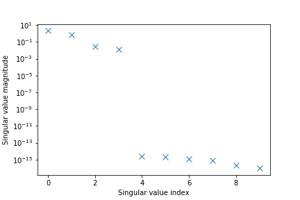
Figure 3: Singular values used to estimate the model order.

In Fig. 3. we can clearly detect a gap between the singular values 4 and 5. This means that 4 is a good estimate of the model order. In fact, this is the exact model order, since our system is of the fourth-order. This graph is generated using
code lines 12-17.

The code lines 19-21 are used to estimate the initial state of the validation data. Namely, to test the model performance, we need to simulate the estimated model using the validation input sequence. However, to perform the simulation,
we need to know the initial states. The identified model has been simulated using the code line 24. The code lines 27-28 are used to compute the relative model error (a relative error measured by the 2-norm between the true validation output and the predicted one).
The code lines 31-37 are used to plot the predicted validation output and the true validation output. The results for several model orders are shown in Figure 4 below.

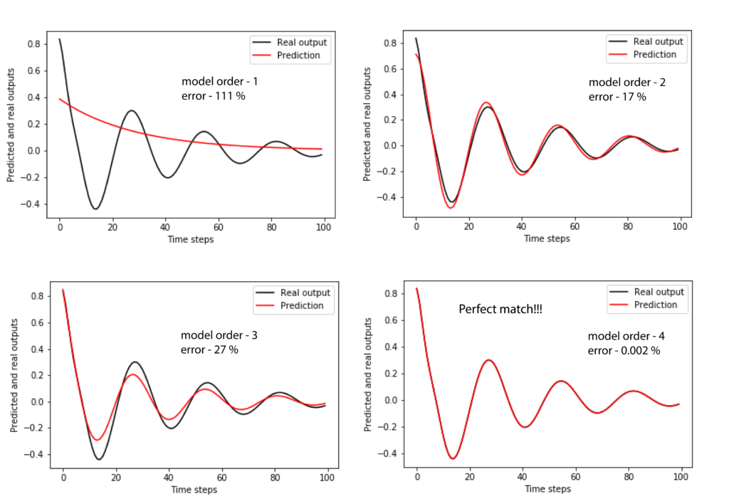
Figure 4: Outputs of the estimated model and the original one for the validation input sequence .

An interesting phenomenon can be observed. Namely, the relative error for the model order of 2 is smaller than the relative error for the model order of 3.

We hope that we have convinced you of the superior performance of the subspace identification algorithms. Notice that we are able to estimate the model by performing only numerical linear algebra steps, without the need to use complex optimization techniques!

Introduction

Test Model – System of Two Objects Connected by Springs and Dampers

Step-by-step Explanation of the Subspace Identification Algorithm

Step 1: Estimation of the VARX model or the System Markov Parameters

Step 2: Estimation of the State-Sequence

Step 3: Estimation of the System Matrices

Model estimation in practice

admin

You might also like

Easy-to-Understand Explanation of Controllable Canonical Form – (also known as Reachable or Control Canonical form)

Ray Tracing with COMSOL – First Part

ROS Tutorial: Create Catkin Workspace and Packages in ROS