Introduction to Model Reference Adaptive Control with MATLAB Simulations – Fusion of Engineering, Control, Coding, Machine Learning, and Science

In this post, we explain how to simulate a model reference adaptive controller in MATLAB. The motivation for creating this post comes from the fact that MATLAB implementation of model reference adaptive controllers is usually omitted in control theory books. However, implementation is far from trivial and there are a number of pitfalls that can potentially lead us to misleading conclusions. In this post, we focus on the adaptive control algorithm whose structure is determined using the so-called MIT rule. An excellent reference to adaptive control is

Åström, K. J., & Wittenmark, B. (2013). Adaptive Control. Courier Corporation.

This post is largely based on Chapter 5 from the above reference. In this post, we numerically simulate Example 5.2 from the above reference. A YouTube video accompanying this post is given here:

A GitHub page with all the codes used in this post can be accessed here.

We focus on a simple first-order system, represented by the differential equation

(1) $\begin{align*}\frac{dy}{dt}=-ay+bu\end{align*}$

where $y$ is an output of the system that we want to control, $u$ is an output of a controller (referred to as the control input), and $a$ and $b$ are constants determining the system dynamics. We assume that constants $a$ and $b$ are unknown during the control design procedure.

The goal of the Model Reference Adaptive Controller (MRAC) is to compute the control input such that the system output is as close as possible to an output of a reference model. The reference model is a model that specifies the desired system behavior. That is, the output of the reference model is the desired system output that we want to achieve in practice. During the design process of MRAC, it is assumed that the reference model is known. Accordingly, for the model (1), the reference model is defined by the following equation

(2) $\begin{align*}\frac{dy_{m}}{dt}=-a_{m}y_{m}+b_{m}u_{c}\end{align*}$

where $y_{m}$ is the output of the reference model, $u_{c}$ is the input of the reference model, and $a_{m}$ and $b_{m}$ are the parameters of the reference model. We assume that $a_{m}$ and $b_{m}$ are known. The signal $u_{c}$ is known. Since $u_{c}$ is known, we can simulate the reference model (2) to generate the output of the reference model $y_{m}$ . The control input structure is given by the following equation

(3) $\begin{align*}u(t)=\theta_{1}(t)u_{c}(t)-\theta_{2}(t)y(t)\end{align*}$

where $\theta_{1}(t)$ and $\theta_{2}(t)$ are the adaptive control parameters that are determined by an adaptive control algorithm.

The goal of the adaptive control algorithm is to determine the parameters $\theta_{1}(t)$ and $\theta_{2}(t)$ such that the system output $y(t)$ is as close as possible to the output $y_{m}(t)$ of the reference model for some selected reference input function $u_{c}(t)$ .

For the development of the control algorithm, it is instructive to perform the following analysis. Namely, by substituting the control law (3) in (1), we obtain

(4) $\begin{align*}\frac{dy}{dt}=-(a+b\theta_{2})y+b\theta_{1}u_{c}\end{align*}$

The model (4) is a closed-loop control system. Let us now compare (4) with the reference model (2). If the parameters $\theta_{1}$ and $\theta_{2}$ take the following constant values

(5) $\begin{align*}\theta_{1}=\theta_{1}^{*}=\frac{b_{m}}{b},\;\; \theta_{2}=\theta_{2}^{*}=\frac{a_{m}-a}{b}\end{align*}$

then, we can conclude that the dynamics of the closed-loop system (4) is identical to the reference model (2). However, in practice, we do not know the constants $a$ and $b$ of the system, and consequently, we cannot determine the parameters $\theta_{1}$ and $\theta_{2}$ in this way. Despite this, the above presented analysis will help us to validate the convergence of the adaptive controller that will be developed in the sequel.

Loosely speaking, the MIT adaptive control rule aims at minimizing the following cost function

(6) $\begin{align*}J=\frac{1}{2}e^{2}\end{align*}$

where $e$ is the control error defined as follows

(7) $\begin{align*}e(t)=y(t)-y_{m}(t)\end{align*}$

To decrease the value of $J$ is reasonable to adjust the parameters $\theta_{1}$ and $\theta_{2}$ in the direction of the negative gradient of J. Using this idea, we obtain

(8) $\begin{align*}\frac{d\theta_{1}}{dt}=-\alpha\frac{\partial J}{\partial \theta_{1}}=-\alpha e\frac{\partial e }{\partial \theta_{1}} \\\frac{d\theta_{2}}{dt}=-\alpha\frac{\partial J}{\partial \theta_{2}}=-\alpha e\frac{\partial e }{\partial \theta_{2}} \end{align*}$

To compute these partial derivatives, we need to express $y(t)$ from (4). This can be done by using a derivative operator $p$ , that acts on a function in the following way

(9) $\begin{align*}pf(t)\equiv \frac{df(t)}{dt}\end{align*}$

Consequently, from (4), we obtain

(10) $\begin{align*}p y =-(a+b\theta_{2})y+b\theta_{1}u_{c} \\(p+a+b\theta_{2})y=b\theta_{1}u_{c} \\y=\frac{b\theta_{1}u_{c}}{p+a+b\theta_{2}} \end{align*}$

Consequently, using (10), the error can be written as follows

(11) $\begin{align*}e=\frac{b\theta_{1}u_{c}}{p+a+b\theta_{2}}-y_{m} \end{align*}$

By taking the partial derivatives of (11) with respect to $\theta_{1}$ and $\theta_{2}$ , we obtain

(12) $\begin{align*}\frac{\partial e }{\partial \theta_{1}}=\frac{bu_{c}}{p+a+b\theta_{2}} \\\frac{\partial e }{\partial \theta_{2}}=\frac{-by}{p+a+b\theta_{2}} \end{align*}$

The partial derivatives in (12) depend on the unknown system parameters $a$ and $b$ and consequently, we cannot explicitly compute them. In order to perform computations, we need to introduce an approximation that is physically justified. Basically, in the ideal scenario, the parameters $\theta_{1}$ and $\theta_{2}$ should converge to the values $\theta_{1}^{*}$ and $\theta_{2}^{*}$ that render the closed-loop dynamics to be equal to the reference model dynamics. In this ideal case, from (5) we have

(13) $\begin{align*}a_{m}=a+b\theta_{2}^{*}\approx a +b\theta_{2} \end{align*}$

Consequently, we can use this approximation to approximate the unknown terms in the denominators of the expressions in (12). Accordingly, we have

(14) $\begin{align*}p+a+b\theta_{2}\approx p+a_{m}\end{align*}$

Next, we substitute this approximation in (12) and as the result, we obtain

(15) $\begin{align*}\frac{\partial e }{\partial \theta_{1}}\approx \frac{bu_{c}}{p+a_{m}} \\\frac{\partial e }{\partial \theta_{2}}\approx \frac{-by}{p+a_{m}}\end{align*}$

Finally, by substituting these partial derivatives in (8) we obtain the final expressions describing parameter changes in time

(16) $\begin{align*} \frac{d\theta_{1}}{dt}=-\underbrace{\alpha\frac{b}{a_{m}}}_{\gamma}\cdot \frac{a_{m}u_{c}}{p+a_{m}}e = -\gamma \frac{a_{m}u_{c}}{p+a_{m}}e \\\frac{d\theta_{2}}{dt}=\underbrace{\alpha\frac{b}{a_{m}}}_{\gamma}\cdot \frac{a_{m}y}{p+a_{m}}e=\gamma \frac{a_{m}y}{p+a_{m}}e \end{align*}$

where $\gamma= \alpha b / a_{m}$ is a new gain. Note that we have normalized the filter

(17) $\begin{align*}\frac{1}{p+a_{m}}\end{align*}$

in this way

(18) $\begin{align*}\frac{a_{m}}{p+a_{m}}\end{align*}$

This filter will now have a unit steady-state gain.

The equations in (16) and the last equation in (10) describe the dynamics of the closed-loop system. These equations are written in the mixed time-domain and differential operator $p$ forms. For further developments, it is instructive to represent these equations in pure time-domain. Using the definition of the differential operator (9) and by performing a few algebraic steps, we obtain

(19) $\begin{align*}\ddot{\theta}_{1}+a_{m}\dot{\theta}_{1}=-\gamma a_{m} u_{c} y+\gamma a_{m} y_{m}u_{c} \\ \ddot{\theta}_{2}+a_{m}\dot{\theta}_{2}=\gamma a_{m} y^{2} - \gamma a_{m} y_{m} y \\\dot{y}= - ay+b\theta_{1}u_{c}-b\theta_{2} y \end{align*}$

where

(20) $\begin{align*}\dot{\theta}_{i}=\frac{d\theta_{i}}{dt},\;\; \ddot{\theta}_{i}=\frac{d\dot{\theta}_{i}}{dt}\end{align*}$

This system of differential equations is coupled with the reference model equation (2) that we rewrite here for clarity.

(21) $\begin{align*}\frac{dy_{m}}{dt}=-a_{m}y_{m}+b_{m}u_{c} \end{align*}$

For selected $u_{c}(t)$ we can simulate the reference model (21). In this way, we obtain the reference model output $y_{m}(t)$ that is a known function of time. The time series $\{u_{c}(t),y_{m}(t) \}$ are used as known “inputs” to steer the dynamics given by (19).

To simulate the model (19), we need to transform it into a state-space model. First, we need to introduce state-space variables:

(22) $\begin{align*}x_{1}=\theta_{1},\; x_{2}=\dot{\theta}_{1},\; x_{3}=\theta_{2},\; x_{4}=\dot{\theta}_{2},\; x_{5}=y\end{align*}$

The state-space model is

(23) $\begin{align*}\dot{x}_{1} &=x_{2} \\\dot{x}_{2} & =-a_{m}x_{2}-\gamma a_{m}u_{c} x_{5}+\gamma a_{m} y_{m} u_{c} \\\dot{x}_{3} &=x_{4} \\\dot{x}_{4} & =-a_{m}x_{4}+\gamma a_{m} x_{5}^{2} - \gamma a_{m} y_{m} x_{5} \\\dot{x}_{5}&=-a x_{5}+bu_{c}x_{1}-bx_{3}x_{5} \end{align*}$

Next, we explain the code for simulating the closed-loop system behavior. We assume the following parameters

(24) $\begin{align*}a_{m}=2,\; b_{m}=2,\; a=1,\; b=0.5\end{align*}$

This combination of parameters gives the following values of the converged parameters (see equations in (5))

(25) $\begin{align*}\theta_{1}^{*}=\frac{2}{0.5}=4,\;\; \theta_{2}^{*}=\frac{2-1}{0.5}=2 \end{align*}$

These values of parameters will be used to verify the convergence of the algorithm.

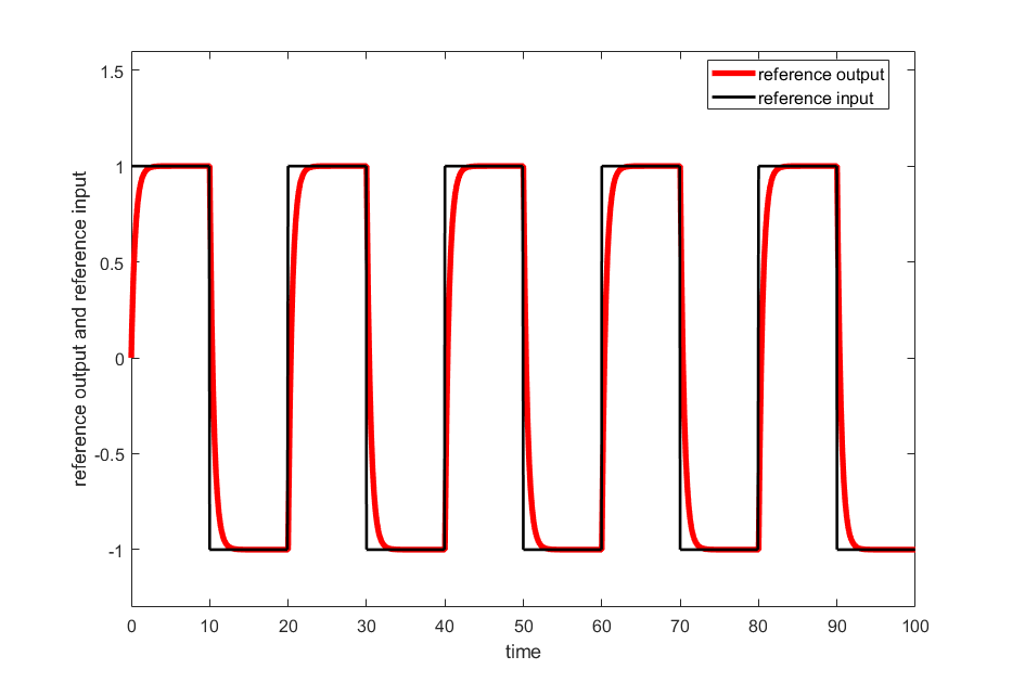
The following code lines are used to define the reference model and to generate the reference input and reference output signals.

% MATLAB simulation of a model reference adaptive controller
% Author: Aleksandar Haber 
% Date: April 21, 2021

% reference model parameters

am=2
bm=2

% plant parameters (that are unknown during control design)
a=1
b=0.5 

%  final values of the parameters for verification of convergence
theta1final=bm/b
theta2final=(am-a)/b

% reference model
Wm=tf([bm],[1 am])

tmax=100 % max simulation time
time=0:0.001:tmax;   %time vector 

% define a reference input signal
pulsew = 10; %pulse width
delayop= pulsew/2:pulsew*2:tmax; %delay vector
% reference input
ur=2*pulstran(time,delayop,'rectpuls',pulsew)-1; 

% input reference signal
figure(1)
plot(time,ur); 
set(gca,'Ylim',[-1.5 1.5]);

% output reference signal
yr=lsim(Wm,ur,time)

figure(2)
plot(time,yr,'r')
hold on
plot(time,ur,'k')

Code line 36 in the above code is used to generate the reference output signal by simulating the reference model.

The reference input and reference output signals are shown in Fig. 1 below.

Figure 1: Reference input and reference output signals obtained by simulating the reference model.

The closed loop system dynamics is defined by the following MATLAB function.

function dxdt = dynamics_adaptive(t, x, um, ym, time_um,am,bm,a,b,gamma)

um_interp = interp1(time_um, um, t); % Interpolate the data set (time_um, um) at time t
ym_interp = interp1(time_um, ym, t); % Interpolate the data set (time_um, ym) at time t

dxdt(1,1)=x(2);
dxdt(2,1)=-am*x(2)-gamma*am*x(5)*um_interp+gamma*am*ym_interp*um_interp;
dxdt(3,1)=x(4);
dxdt(4,1)=-am*x(4)+gamma*am*x(5)^2-gamma*am*x(5)*ym_interp;
dxdt(5,1)=-a*x(5)+b*x(1)*um_interp-b*x(3)*x(5);

This function takes as input the current time “t”, current state “x”, reference model control input vector “um”, reference model output vector “ym”, time vector “time_um”, parameters “am”,”bm”,”a”,”b”, and the control gain “gamma”. This function is a MATLAB implementation of the closed-loop system dynamics given by (23).
We use an interpolation approach for dealing with time-varying inputs “um” and “ym” in ode45 function simulations. More details about this approach can be found in this and in this posts.

The state trajectories are simulated by executing these lines of code.

% initial condition
x0=zeros(5,1);
% gain
gamma2=0.5;

[time1 state_trajectories] = ode45(@(t,x) dynamics_adaptive(t, x, ur, yr, time,am,bm,a,b,gamma2), time, x0);

theta1=state_trajectories(:,1)
theta2=state_trajectories(:,3)
y=state_trajectories(:,5)


figure(3)
plot(time,yr,'k')
hold on
plot(time,y,'m')

figure(4)
plot(time,theta1,'k')
hold on 
plot(time,theta2,'m')

We simulate the system response for three values of the controller gain $\gamma=0.5$ , $\gamma=2$ , and $\gamma=4$ .

The reference model output and the controlled output of the plant are shown in Fig. 2 for $\gamma=0.5$ .

Figure 2: The reference model output and the controlled output of the plant for $\gamma=0.5$ .

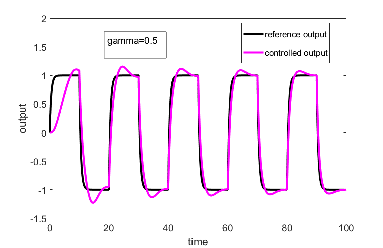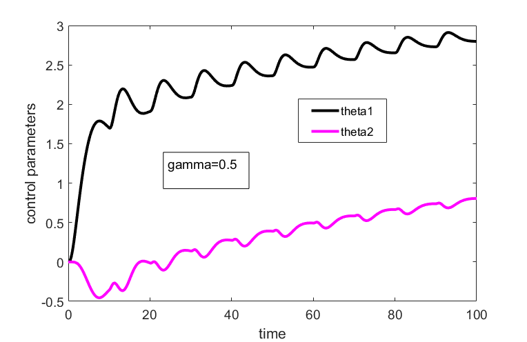
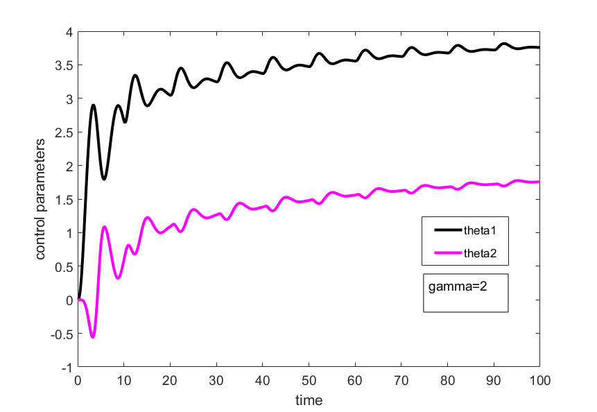
The convergence trajectories of the parameters $\theta_{1}$ and $\theta_{2}$ are shown in Fig. 3 for $\gamma = 0.5$ .

Figure 3: Trajectories of the parameters $\theta_{1}$ and $\theta_{2}$ for $\gamma=0.5$ .

The reference model output and the controlled output of the plant are shown in Fig. 4 for $\gamma=2$ .

*Figure 4: The reference model output and the controlled output of the plant for $\gamma=2$ .*

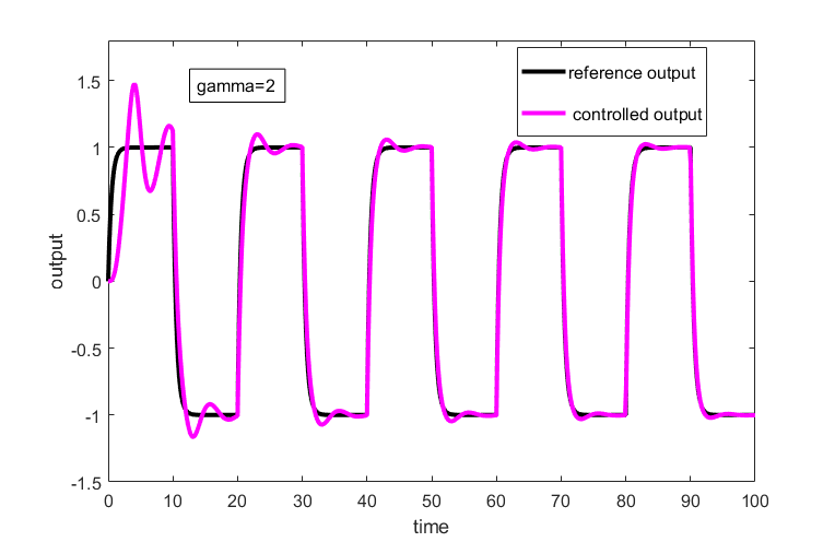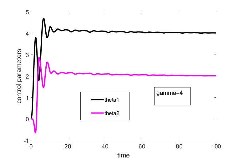
The convergence trajectories of the parameters $\theta_{1}$ and $\theta_{2}$ are shown in Fig. 5 for $\gamma = 2$ .

*Figure 5: Trajectories of the parameters $\theta_{1}$ and $\theta_{2}$ for $\gamma=2$* .

The reference model output and the controlled output of the plant are shown in Fig. 6 for $\gamma=4$ .

*Figure 6: The reference model output and the controlled output of the plant for $\gamma=4$ .*

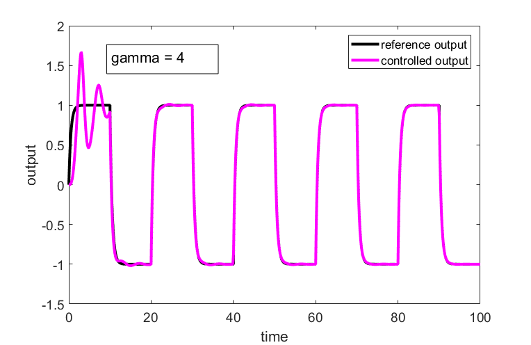The convergence trajectories of the parameters $\theta_{1}$ and $\theta_{2}$ are shown in Fig. 7 for $\gamma = 4$ .

*Figure 7: Trajectories of the parameters $\theta_{1}$ and $\theta_{2}$ for $\gamma=4$ .*

From figures 2-7, we can conclude the following

The convergence of the parameters increases for larger values of $\gamma$ . For $\gamma=4$ the parameters $\theta_{1}$ and $\theta_{2}$ approximately converge in 20 seconds to the values $\theta_{1}^{*}$ and $\theta_{2}^{*}$ . This shows that the controller works well and that the equations are properly implemented.
After the initial transients difference between the controlled output and the reference model output decreases as we increase $\gamma$ . However, for larger values of $\gamma$ the control transients start to exhibit oscillatory behavior. This can be seen during the first 10 seconds in Figs. 4 and 6. Increased overshoot is the price we need to pay for achieving a better tracking performance.

admin

You might also like

Test 3

Optional Homework Assignment: Solving beam differential equation in the reversed coordinate system

Python Implementation of the Greedy in the Limit with Infinite Exploration (GLIE) Monte Carlo Control Method – Reinforcement Learning Tutorial with OpenAI Gym