Python Implementation of the Greedy in the Limit with Infinite Exploration (GLIE) Monte Carlo Control Method – Reinforcement Learning Tutorial with OpenAI Gym – Fusion of Engineering, Control, Coding, Machine Learning, and Science

In this reinforcement learning tutorial, we explain how to implement the Greedy in the Limit with Infinite Exploration (GLIE) Monte Carlo Control Method in Python. The GitHub page with all the codes is given here.

Before reading this tutorial, it is suggested that you go over the previous tutorials and topics:

Clear Explanation of the Value Function and Its Bellman Equation – Reinforcement Learning Tutorial
Installation and Getting Started with OpenAI Gym and Frozen Lake Environment – Reinforcement Learning Tutorial
Policy Iteration Algorithm in Python and Tests with Frozen Lake OpenAI Gym Environment- Reinforcement Learning Tutorial
Monte Carlo Method for Learning State-Value Functions – First Visit Method – Reinforcement Learning Tutorial

The Main Idea of the GLIE Monte Carlo Control Method

In this tutorial, we denote the action value function by $q(s,a)$ , where $s$ is the current state, and $a$ is the action taken at the current state. The GLIE Monte Carlo control method is a model-free reinforcement learning algorithm for learning the optimal control policy.

The main idea of the GLIE Monte Carlo control method can be summarized as follows.

Use the Monte Carlo method to learn action value function $q(s,a)$ . This is done by running a learning episode, observing the states, actions, and rewards, and on the basis of this collected data updating the estimate $q(s,a)$ . The estimates are computes as averages, as explained in this post, except for the fact that the averaging is applied to the action value function, instead of the state value function.
In every learning episode, we use an epsilon greedy approach to select the actions on the basis of the current estimate of the action-value function.

By using this procedure, we can learn the optimal policy.

First, let us explain the epsilon greedy approach for selecting an action. Let us consider the OpenAI Frozen Lake environment which we explained in this tutorial. This environment is illustrated in the figure 1 below.

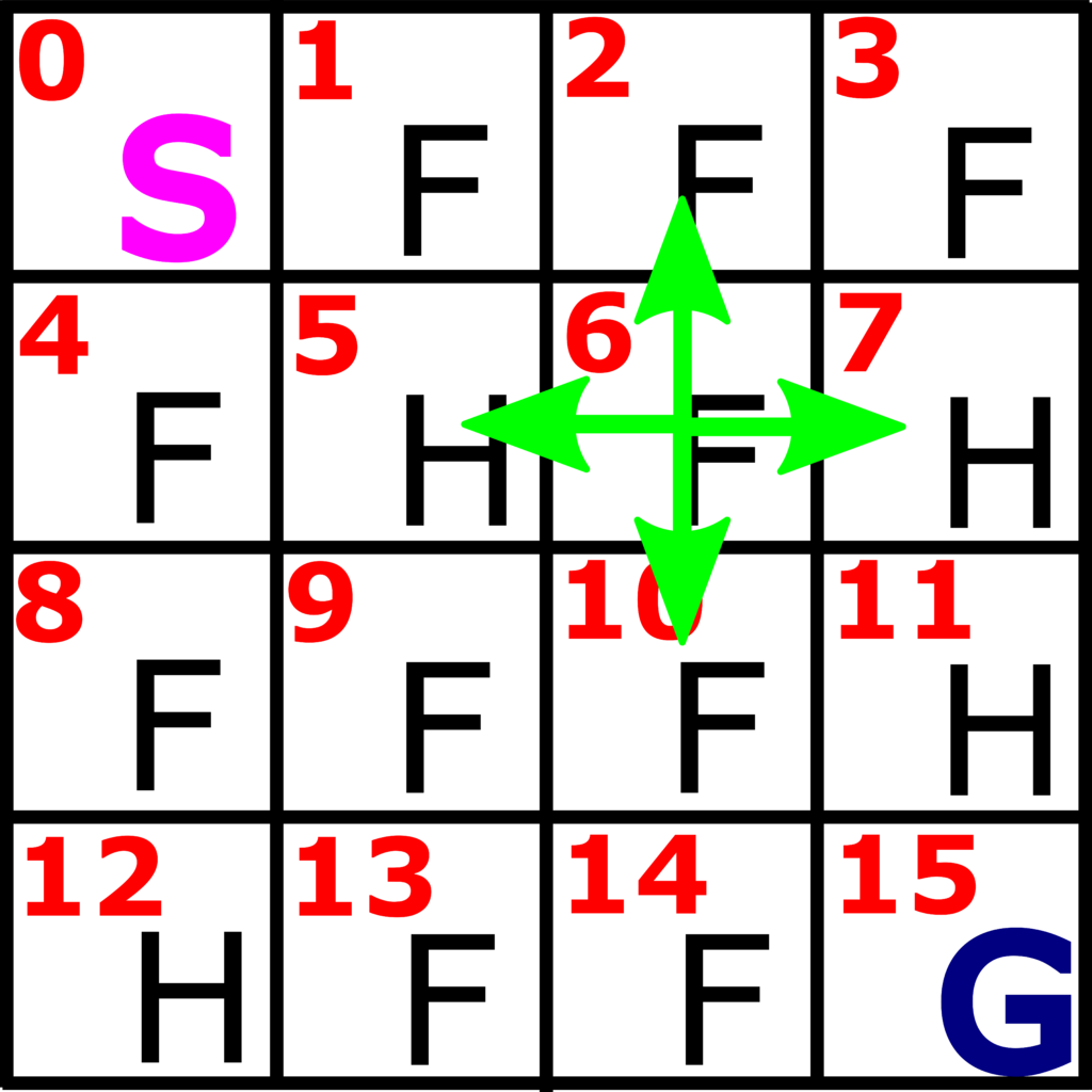
Let us suppose that we are in the state 6, and let us assume that the current estimate in the state 6 is

(1) $\begin{align*}q(6,a)=\begin{bmatrix} 0.25 & 0.6 & 0 & 0.25\end{bmatrix}\end{align*}$

where the column numbers of this vector (starting from zero in order to be consistent with the Python notation) correspond to the actions: 0 column is left, column 1 is action “down”, column 2 is action “right”, and column 3 is action “up”. The greedy action selection will select the action with the column number 1, corresponding to the maximal value of the action value function. That is, the maximum is $q(6,1)=0.6$ and it is achieved for the action 1. Consequently, we choose the action $1$ . This is the main idea of the greedy approach. In every state, select an action that produces the maximum value of the action value function. However, this greedy approach has one drawback. For example, let us suppose that we run the algorithm from the first episode. In this first episode, we randomly select actions since there is no previously computed data on which basis we can estimate $q(s,a)$ . We assume that the initial value of $q(s,a)$ is zero for all the states and actions. Then, after the first episode is completed, we can obtain an estimate of $q(s,a)$ for the visited states. Now, if we follow the greedy approach, in the second interaction we will select the actions that are taken in the first iteration. This is because in the first iteration, only pairs (s,a) that are visited are non-zero and all other pairs are zero. Due to this, the same set of actions will be selected in all subsequent episodes. Consequently, we might not be able to compute the optimal policy.

This problem motivates the epsilon-greedy policy. In the epsilon greedy policy, we do the following. First, we select a small number $\varepsilon <1$ (let us say smaller than 0.3)

Draw a random number from 0 to 1.
If this number is smaller than a user-defined number $\varepsilon$ , then we randomly select an action in a certain state $s$ .
On the other hand, if this number is larger than $\varepsilon$ , we select an action that maximizes the action value function in the particular state.

This is the epsilon-greedy learning approach. It enables us to deviate from the greedy approach by performing exploration. Exploration is a fancy word used to denote random actions. Now in practice, we use an epsilon greedy approach for the first let us say $n$ episodes, and after $n$ after which we learn the environment model sufficiently accurately, we need to start decreasing $\varepsilon$ gradually. This can for example be achieved as follows

(2) $\begin{align*}\varepsilon \rightarrow k \cdot \varepsilon,\;\; k<1 , \;\; \text{after n episodes}\end{align*}$

In this way, we ensure that after we learn the model sufficiently accurately, we start to explore less and less in order to ensure that we converge to the static policy.

Before we implement the Monte Carlo method, we need to derive a recursive formula for averages. Consider this average of the numbers $x_{1}$ , $x_{2}$ , …, $x_{l}$ collected until and including an iteration $l$ . Then the average is given by:

(3) $\begin{align*}\bar{x}_{l}=\frac{\Sigma_{l}}{l}=\frac{x_{1}+x_{2}+\ldots +x_{l}}{l} \\\Sigma_{l}= x_{1}+x_{2}+\ldots +x_{l}\end{align*}$

This average can be expressed as follows

(4) $\begin{align*}\bar{x}_{l} & =\frac{\Sigma_{l-1}+x_{l}}{l}=\frac{\bar{x}_{l-1}(l-1)+x_{l}}{l} \\& = \bar{x}_{l-1}+\frac{1}{l}(x_{l}- \bar{x}_{l-1})\end{align*}$

Since in the Monte Carlo method, the action value functions are estimated as averages, we can use this recursive formula to estimate them without storing the sums.

Python Code Implementing the GLIE Monte Carlo Control Method

The GitHub page with all the codes is given here.

We use the Frozen lake environment to test the Monte Carlo method. The function below implements the GLIE Monte Carlo Control method. Later on, we give a driver code for this function.

# -*- coding: utf-8 -*-
"""
Python Implementation of 
the Greedy in the Limit with Infinite Exploration (GLIE) Monte Carlo Control Method

Author: Aleksandar Haber 
Date: December 2023
"""


###############################################################################
# this function learns the optimal policy by using the GLIE Monte Carlo Control Method
###############################################################################
# inputs: 
##################
# env - OpenAI Gym environment 
# stateNumber - number of states
# numberOfEpisodes - number of simulation episodes
# discountRate - discount rate 
# initialEpsilon - initial value of epsilon for the epsilon greedy approach
##################
# outputs:
##################
# finalPolicy - learned policy 
# actionValueMatrixEstimate - estimate of the action value function matrix
##################

def MonteCarloControlGLIE(env,stateNumber,numberOfEpisodes,discountRate,initialEpsilon):
    ###########################################################################
    #                   START - parameter definition
    ###########################################################################
    import numpy as np
    # number of actions in every state 
    actionNumber=4
    # initial epsilon-greedy parameter
    epsilon=initialEpsilon
    # this matrix stores state-action visits
    # that is in state i, action j is selected, then (i,j) entry of this matrix
    # incremented
    numberVisitsForEveryStateAction=np.zeros((stateNumber,actionNumber))
    # estimate of the action value function matrix 
    # initial value
    actionValueMatrixEstimate=np.zeros((stateNumber,actionNumber))
    # final learned policy, it is an array of stateNumber entries
    # every entry of the list is the action selected in that state
    finalPolicy=np.zeros(stateNumber)
    ###########################################################################
    #                   END - parameter definition
    ###########################################################################
    
    ###########################################################################
    #    START - function selecting an action: epsilon-greedy approach
    ###########################################################################
    # this function selects an action on the basis of the current state 
    def selectAction(state,indexEpisode):
        
        # first 5 episodes we select completely random actions to avoid being stuck
        if indexEpisode<5:
            return np.random.choice(actionNumber)   
            
             
        # Returns a random real number in the half-open interval [0.0, 1.0)
        randomNumber=np.random.random()
            
        
        
        # if this condition is satisfied, we are exploring, that is, we select random actions
        if randomNumber < epsilon:
            # returns a random action selected from: 0,1,...,actionNumber-1
            return np.random.choice(actionNumber)            
        
        # otherwise, we are selecting greedy actions
        else:
            # we return the index where actionValueMatrixEstimate[state,:] has the max value
            return np.random.choice(np.where(actionValueMatrixEstimate[state,:]==np.max(actionValueMatrixEstimate[state,:]))[0])
            # here we need to return the minimum index since it can happen
            # that there are several identical maximal entries, for example 
            # import numpy as np
            # a=[0,1,1,0]
            # np.where(a==np.max(a))
            # this will return [1,2], but we only need a single index
            # that is why we need to have np.random.choice(np.where(a==np.max(a))[0])
            # note that zero has to be added here since np.where() returns a tuple
    ###########################################################################
    #    END - function selecting an action: epsilon-greedy approach
    ###########################################################################
    
    
    ###########################################################################
    # START - outer loop for simulating episodes
    ###########################################################################
    for indexEpisode in range(numberOfEpisodes):
        
        # this list stores visited states in the current episode
        visitedStatesInEpisode=[]
        # this list stores the return in every visited state in the current episode
        rewardInVisitedState=[]
        # selected actions in an episode 
        actionsInEpisode=[]
        # reset the environment at the beginning of every episode
        (currentState,prob)=env.reset()
        visitedStatesInEpisode.append(currentState)
        print("Simulating episode {}".format(indexEpisode))
         
         
        ###########################################################################
        # START - single episode simulation
        ###########################################################################
        # here we simulate an episode
        while True:
             
            # select an action on the basis of the current state
            selectedAction = selectAction(currentState, indexEpisode)
            # append the selected action
            actionsInEpisode.append(selectedAction)
                         
            # explanation of "env.action_space.sample()"
            # Accepts an action and returns either a tuple (observation, reward, terminated, truncated, info)
            # https://www.gymlibrary.dev/api/core/#gym.Env.step
            # format of returnValue is (observation,reward, terminated, truncated, info)
            # observation (object)  - observed state
            # reward (float)        - reward that is the result of taking the action
            # terminated (bool)     - is it a terminal state
            # truncated (bool)      - it is not important in our case
            # info (dictionary)     - in our case transition probability
            # env.render()
             
            # here we step and return the state, reward, and boolean denoting if the state is a terminal state
            (currentState, currentReward, terminalState,_,_) = env.step(selectedAction)          
            #print(currentState,selectedAction)
            # append the reward
            rewardInVisitedState.append(currentReward)
             
            # if the current state is NOT terminal state 
            if not terminalState:
                visitedStatesInEpisode.append(currentState)   
            # if the current state IS terminal state 
            else: 
                break
            # explanation of IF-ELSE:
            # let us say that a state sequence is 
            # s0, s4, s8, s9, s10, s14, s15
            # the vector visitedStatesInEpisode is then 
            # visitedStatesInEpisode=[0,4,8,10,14]
            # note that s15 is the terminal state and this state is not included in the list
             
            # the return vector is then
            # rewardInVisitedState=[R4,R8,R10,R14,R15]
            # R4 is the first entry, meaning that this is the reward going
            # from state s0 to s4. That is, the rewards correspond to the reward
            # obtained in the destination state
         
        ###########################################################################
        # END - single episode simulation
        ###########################################################################
         
        ###########################################################################
        # START - updates of the action value function and number of visits
        ########################################################################### 
        # how many states we visited in an episode    
        numberOfVisitedStates=len(visitedStatesInEpisode)
             
        # this is Gt=R_{t+1}+\gamma R_{t+2} + \gamma^2 R_{t+3} + ...
        Gt=0
        # we compute this quantity by using a reverse "range" 
        # below, "range" starts from len-1 until second argument +1, that is until 0
        # with the step that is equal to the third argument, that is, equal to -1
        # here we do everything backwards since it is easier and faster 
        # if we go in the forward direction, we would have to 
        # compute the total return for every state, and this will be less efficient
         
        for indexCurrentState in range(numberOfVisitedStates-1,-1,-1):
            
            stateTmp=visitedStatesInEpisode[indexCurrentState] 
            returnTmp=rewardInVisitedState[indexCurrentState]
            actionTmp=actionsInEpisode[indexCurrentState]
            # this is an elegant way of summing the returns backwards 
            Gt=discountRate*Gt+returnTmp
            # below is the first visit implementation 
            if stateTmp not in visitedStatesInEpisode[0:indexCurrentState]:
                
                numberVisitsForEveryStateAction[stateTmp,actionTmp]+=1
                actionValueMatrixEstimate[stateTmp,actionTmp]=actionValueMatrixEstimate[stateTmp,actionTmp]+(1/numberVisitsForEveryStateAction[stateTmp,actionTmp])*(Gt-actionValueMatrixEstimate[stateTmp,actionTmp])
        ###########################################################################
        # END - updates of the action value function and number of visits
        ########################################################################### 
        
        # first 100 episodes, we keep a fixed value of 
        # epsilon to ensure that we explore enough
        # after that, we decrease the epsilon value
        if indexEpisode < 1000:
            epsilon=initialEpsilon
        else:
            epsilon=0.8*epsilon
        
            
    ###########################################################################
    # END - outer loop for simulating episodes
    ###########################################################################
        
    # now we compute the final learned policy
    for indexS in range(stateNumber):
        # we use np.random.choice() because in theory, we might have several identical maximums
        finalPolicy[indexS]=np.random.choice(np.where(actionValueMatrixEstimate[indexS]==np.max(actionValueMatrixEstimate[indexS]))[0])
        
     
    return finalPolicy,actionValueMatrixEstimate

This function deliberately contains a number of comments in order to make it more readable and accessible.

The function takes the following input arguments: 1) environment, 2) the number of states of the environment (16 in our case since we are considering the Frozen lake environment), 3) number of simulation episodes, 4) discount rate, and 5) initial value of the epsilon parameter. This function returns the final learned policy. This final learned policy is a vector with a dimension equal to the number of states. Every entry of this function is the action that has to be taken in a certain state. Also, this function returns the matrix with estimated action-value functions. This matrix is used for inspection purposes and diagnosis.

The code lines 40-46 define

Matrix “numberVisitsForEveryStateAction” contains the number of visits of the pair (s,a), where s is the state index (0 to 15- we have 16 states) and a is an action index ( from 0 to 3), during episode simulations.
Matrix “actionValueMatrixEstimate”. The entry (s,a) of this matrix is the estimated value of the action value function that is usually denoted by q(s,a).
Vector “finalPolicy” with the dimension equal to the number of states. This is the final policy that we are learning. Entry s of this vector is the action we need to take (action numbers are from 0 to 3).

The function defined on the code lines from 55 to 83 is used to select the action by using the epsilon greedy method. Note here that during the first 5 episode simulations, we select random control actions in order to ensure that we have enough random explorations before the epsilon-greedy algorithm becomes active.

The for loop defined on the code lines 92 to 197 is used to simulate episodes. On the code line 101, we reset the environment to make sure that every episode starts from the same state (you can also relax that, by choosing a random initial state). The while loop starting at the code line 110 and ending at the code line 153 is used to simulate a single episode. This while loop is broken if we reach the terminal state (either the goal state of the hole state of the Frozen Lake environment). On the code line 113, we select a control action by calling the previously defined function “selectAction()”. On the code line 129 we apply the control action, and observe the destination state and the obtained reward. The code lines 161 to 184 are used to estimate the matrix “actionValueMatrixEstimate” by using the previously explained recursive formula for computing the averages. The code lines 191 to 194 are used to control the value of $\varepsilon$ . Finally, the code lines 202 to 204 are used to compute the final policy.

The driver code that demonstrates how to use this function is given below.

'''
Python Implementation of 
the Greedy in the Limit with Infinite Exploration (GLIE) Monte Carlo Control Method

Author: Aleksandar Haber

'''
# Note: 
# You can either use gym (not maintained anymore) or gymnasium (maintained version of gym)    
    
# tested on     
# gym==0.26.2
# gym-notices==0.0.8

#gymnasium==0.27.0
#gymnasium-notices==0.0.1

# classical gym 
import gym
# instead of gym, import gymnasium 
# import gymnasium as gym

import matplotlib.pyplot as plt
import seaborn as sns
import numpy as np
import time
from functions import MonteCarloControlGLIE
 
# create the environment 
# is_slippery=False, this is a completely deterministic environment, 
# uncomment this if you want to render the environment during the solution process
# however, this will slow down the solution process
#env=gym.make('FrozenLake-v1', desc=None, map_name="4x4", is_slippery=False,render_mode="human")

# here we do not render the environment for speed purposes
env=gym.make('FrozenLake-v1', desc=None, map_name="4x4", is_slippery=False)
env.reset()
# render the environment
# uncomment this if you want to render the environment
#env.render()
# this is used to close the rendered environment
#env.close()
 
# investigate the environment
# observation space - states 
env.observation_space
 
env.action_space
# actions:
#0: LEFT
#1: DOWN
#2: RIGHT
#3: UP
 
# general parameters for the Monte Carlo method
# select the discount rate
discountRate=0.9
# number of states - determined by the Frozen Lake environment
stateNumber=16
# number of possible actions in every state - determined by the Frozen Lake environment
actionNumber=4
# maximal number of iterations of the policy iteration algorithm 
numberOfEpisodes=10000
# initial value of epsilon
initialEpsilon=0.2
# learn the optimal policy
finalLearnedPolicy,Qmatrix=MonteCarloControlGLIE(env,stateNumber,numberOfEpisodes,discountRate,initialEpsilon)

# to interpret the final learned policy you need this information
# actions: 0: LEFT, 1: DOWN, 2: RIGHT, 3: UP
# let us simulate the learned policy
# this will reset the environment and return the agent to the initial state
env=gym.make('FrozenLake-v1', desc=None, map_name="4x4", is_slippery=False,render_mode='human')
(currentState,prob)=env.reset()
env.render()
time.sleep(2)
# since the initial state is not a terminal state, set this flag to false
terminalState=False
for i in range(100):
    # here we step and return the state, reward, and boolean denoting if the state is a terminal state
    if not terminalState:
        (currentState, currentReward, terminalState,_,_) = env.step(int(finalLearnedPolicy[currentState]))
        time.sleep(1)
    else:
        break
time.sleep(2)
env.close()

First, we import the necessary libraries. Here it should be noted that we can either use Gym or Gymnasium library. The Gymnasium library is a maintained fork of the OpenAI Gym. Then, we define the necessary parameters and call the function MonteCarloControlGLIE which implements the GLIE Monte Carlo method. Once an estimate of the optimal policy is computed, we simulate and visualize the policy on code lines 73 to 87.

The Main Idea of the GLIE Monte Carlo Control Method

Python Code Implementing the GLIE Monte Carlo Control Method

admin

You might also like

Fanuc Robot Coding: Jump and Label instructions

Matrix Exponential Tutorial: Definition, Calculation, and its Application in Control Engineering and Control Theory – PART 1

Generate PWM signals in STM32 microcontrollers