Interpolation of Function Values in MATLAB

In this post, we explain how to interpolate function values in MATLAB. The goal is to generate function values at predefined coarse-spaced points and then to interpolate the values of this function at the denser grid of points. The Youtube video accompanying this post is given below.

Accordingly, we first define coarse and dense grids of values on the x axis. The code is given below

% function interpolation in MATLAB
clear, pack, clc

step_coarse=0.4
step_dense=0.2
final_time=10

time_coarse=0:step_coarse:final_time
time_dense=0:step_dense:final_time

The vectors “time_coarse” and “time_dense” are used to store coarse and dense grids of points on the x axis. In this post, we interpolate the values of the following function

(1)  

where is time (independent variable that is plotted on the x axis). The following code lines are used to define this function and to interpolate its values. Also, we plot the original function and its interpolated values defined on a denser grid of points.

% coarse function to interpolate
coarse_function=time_coarse.^2-0.1*time_coarse.^3

% Vq = interp1(X,V,Xq) interpolates to find Vq, the values of the underlying function V=F(X) at the query points Xq. 
dense_function_interpolated = interp1(time_coarse,coarse_function,time_dense);

figure(1)
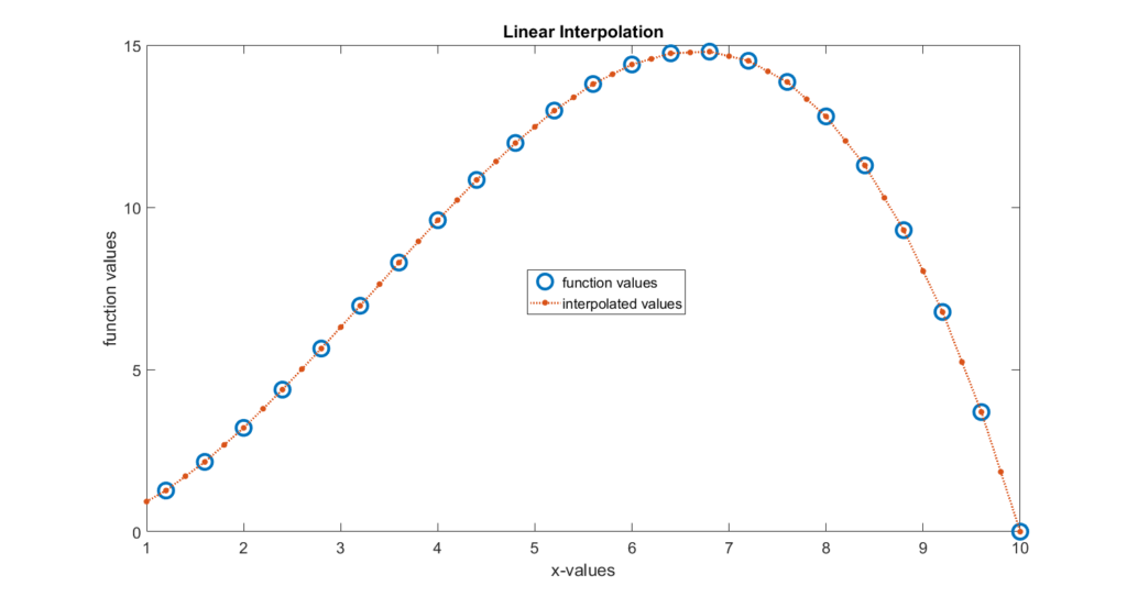
plot(time_coarse,coarse_function,'o',time_dense,dense_function_interpolated,':.');
xlim([1 10]);
title('Linear Interpolation');

The MATLAB function “interp1()” is used to interpolate the function values. The first two arguments are the set of points that define the original function. In our case, the first two arguments are “time_coarse” and “coarse_function” which are used to define the original function values. The third argument is a set of values on the x axis at which we want to compute the interpolated values. In our case, this vector is called “time_dense”. The results are given in Fig. 1 below.

The MATLAB function “interp1()” computes interpolated values using the default settings that correspond to linear interpolation. If we want to perform some other type of interpolation, we need to specify the fourth argument. If we type “help interp1” we can obtain the following options.

Vq = interp1(X,V,Xq,METHOD) specifies the interpolation method.
    The available methods are:
 
      'linear'   - (default) linear interpolation
      'nearest'  - nearest neighbor interpolation
      'next'     - next neighbor interpolation
      'previous' - previous neighbor interpolation
      'spline'   - piecewise cubic spline interpolation (SPLINE)
      'pchip'    - shape-preserving piecewise cubic interpolation
      'cubic'    - same as 'pchip'
      'v5cubic'  - the cubic interpolation from MATLAB 5, which does not
                   extrapolate and uses 'spline' if X is not equally
                   spaced.

For example, we can compute cubic interpolation by executing the following code lines.

% 'pchip'    - shape-preserving piecewise cubic interpolation
% Vq = interp1(X,V,Xq,METHOD)
dense_function_interpolated_cubic = interp1(time_coarse,coarse_function,time_dense,'pchip');

figure(2)
plot(time_coarse,coarse_function,'o',time_dense,dense_function_interpolated_cubic,':.');
xlim([1 10]);
title('Cubic Interpolation');