Clear and Concise Explanation of Fourier Series With Solved Examples and Python code – Fusion of Engineering, Control, Coding, Machine Learning, and Science

In this mathematics, signal processing, and control engineering tutorial, we provide a clear and concise explanation of the Fourier series. In addition, we solve several examples in order to illustrate how to compute Fourier series. The main goal of this tutorial is to provide a very concise, self-contained, and clear tutorial on the Fourier series, such that students and engineers can quickly grasp the main ideas and obtain a proper understanding of the Fourier series. Also, the idea is to clarify a few misconceptions about the Fourier series and to solve several examples that can help students to better understand the mathematics behind the Fourier series. Finally, we provide Python scripts for computing the coefficients of the Fourier expansion. The YouTube tutorial accompanying this tutorial is given below.

Basics of Fourier Series and Main Formulas

The main idea of the Fourier series is to represent a periodic function as an infinite or finite sum of harmonic signals ( $\sin$ and $\cos$ functions). We can also use the Fourier series for periodic extensions of non-periodic functions.

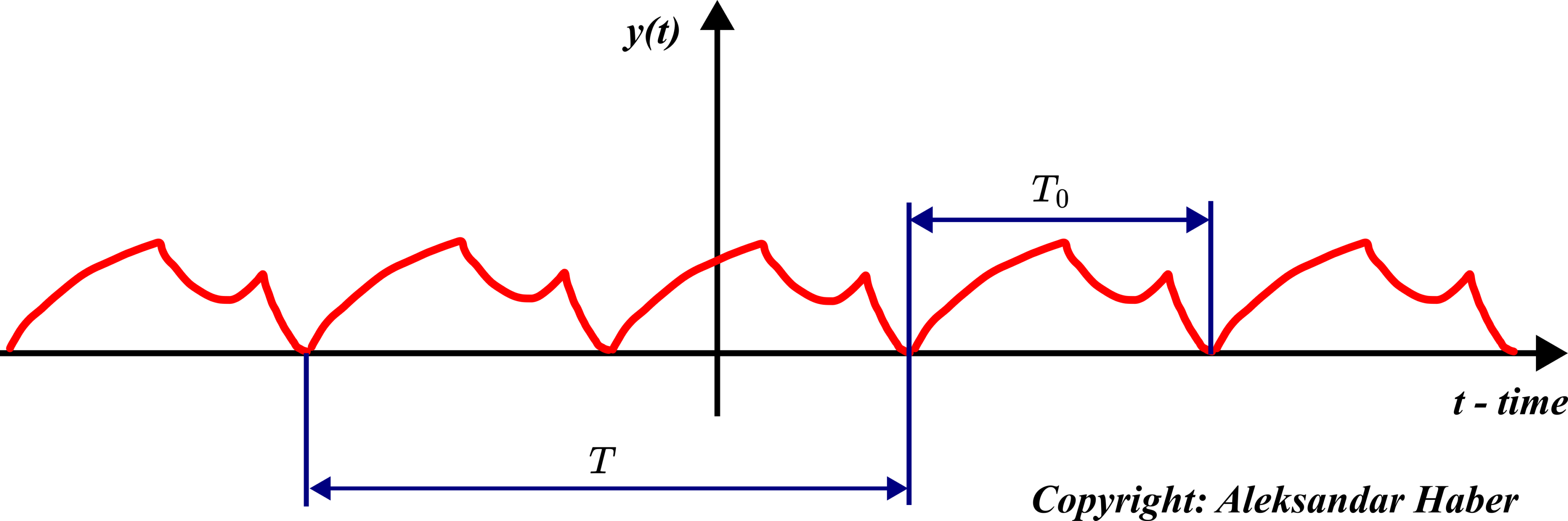
However, before we state the main formulas of the Fourier series, we need to introduce a few important concepts. Consider the figure shown below.

Figure 1: Periodic signal with the period of $T$ and with the fundamental period of $T_{0}$ .

This figure shows a periodic function. Formally speaking, the function $y(t)$ is periodic if and only if there exists a real positive number $T$ such that

(1) $\begin{align*}y(t)=y(t+T)\end{align*}$

where $T>0$ is called the period of the function. That is, the periodic function repeats itself after $T$ seconds. Now, we are ready to define two very important concepts:

The fundamental period, denoted by $T_{0}$ , is the smallest positive real number $T$ for which the equation (1) is satisfied. The fundamental period is illustrated in Fig. 1. above.
By using the fundamental period, we define the fundamental frequency $\omega_{0}$ as follows
(2) $\begin{align*}\omega_{0}=\frac{2\pi }{T_{0}}\end{align*}$

The Fourier series of a periodic function $y(t)$ is defined by the following infinite sum

(3) $\begin{align*}y(t)=\sum_{k=-\infty}^{+\infty} c_{k}e^{jk\omega_{0}t}\end{align*}$

where $j$ is the imaginary unit, and the Fourier series coefficients $c_{k}$ are defined as

(4) $\begin{align*}c_{k}=\frac{1}{T_{0}}\int_{T_{0}}y(t)e^{-jk\omega_{0}t} \mathrm{d}t\end{align*}$

The Fourier series form presented above is called the complex form of the Fourier series. Besides this form, there are a number of equivalent mathematical forms that are derived from this form. For signal processing and control engineering, the complex form is the most useful one. In our future tutorials, we will explain other forms.

In the sequel, we provide a more intuitive explanation of the Fourier series. First of all, to better understand the sum (3), let us write first several terms

(5) $\begin{align*}y_{2}(t) & =c_{-2}e^{-j2\omega_{0}t}+c_{-1}e^{-j\omega_{0}t}+c_{0}e^{-j0\omega_{0}t} \\& +c_{1}e^{j\omega_{0}t}+c_{2}e^{-j2\omega_{0}t}\end{align*}$

On the other hand, let us recall Euler’s formula for the exponential of the complex number:

(6) $\begin{align*}e^{j\theta}=\cos(\theta)+j\sin (\theta)\end{align*}$

From this formula, we can see that every complex exponential in (5) or in the general equation (3) can be represented as a sum of $\sin$ and $\cos$ functions. Consequently, the Fourier series expansion consists of sums of $\sin$ and $\cos$ functions with different frequencies that are multiples of the fundamental frequency $\omega_{0}$ .

Now, let us explain what are the DC gain, fundamental component, and harmonics.

The DC component of the function (signal) $y(t)$ is the Fourier series coefficient $c_{0}$ :
(7) $\begin{align*}c_{0}=\frac{1}{T_{0}}\int_{T_{0}}y(t)\mathrm{d}t\end{align*}$

This is simply an average of the function $y(t)$ over the fundamental period $T_{0}$ .
The elements of the Fourier series expansion obtained for $k=1$ or $k=-1$ are called the fundamental components or the first harmonic components or simply, first harmonics. That is, the following elements are the fundamental components or first harmonics:
(8) $\begin{align*}c_{1}e^{j\omega_{0}t},\;\;\; c_{-1}e^{-j\omega_{0}t}\end{align*}$
The components obtained for $k=\pm n$ are called the $n$ th harmonic components or simply $n$ th harmonics. That is, the $n$ th harmonics are defined by
(9) $\begin{align*}c_{n}e^{jn\omega_{0}t},\;\;\; c_{-n}e^{-jn\omega_{0}t}\end{align*}$

Before we proceed with examples, one very important thing about Fourier series expansion needs to be emphasized. Namely, the coefficients $c_{k}$ and $c_{-k}$ are related. From the equation (4), it follows that

(10) $\begin{align*}c_{k}^{*}=c_{-k}\end{align*}$

where $*$ operator is the complex conjugateHere, we give a graphical example of the Fourier series. The goal is to approximate a periodic rectangular wave. In the sequel of this tutorial, we will derive a formula for the Fourier series coefficients of this function. For the time being, we only graphically show the approximation for different values of $k$ . The figure below shows the approximation of the wave for $k=0,\pm 1$ . That is, we only take into account the DC component and the fundamental components. For the fundamental period of $T_{0}=4$ , the approximation is

(11) $\begin{align*}\left(0.31831 - 0.31831 i\right) e^{\frac{i \pi t}{2}} + 0.5 + \left(0.31831 + 0.31831 i\right) e^{- \frac{i \pi t}{2}}\end{align*}$

and figure below shows the graphical representation

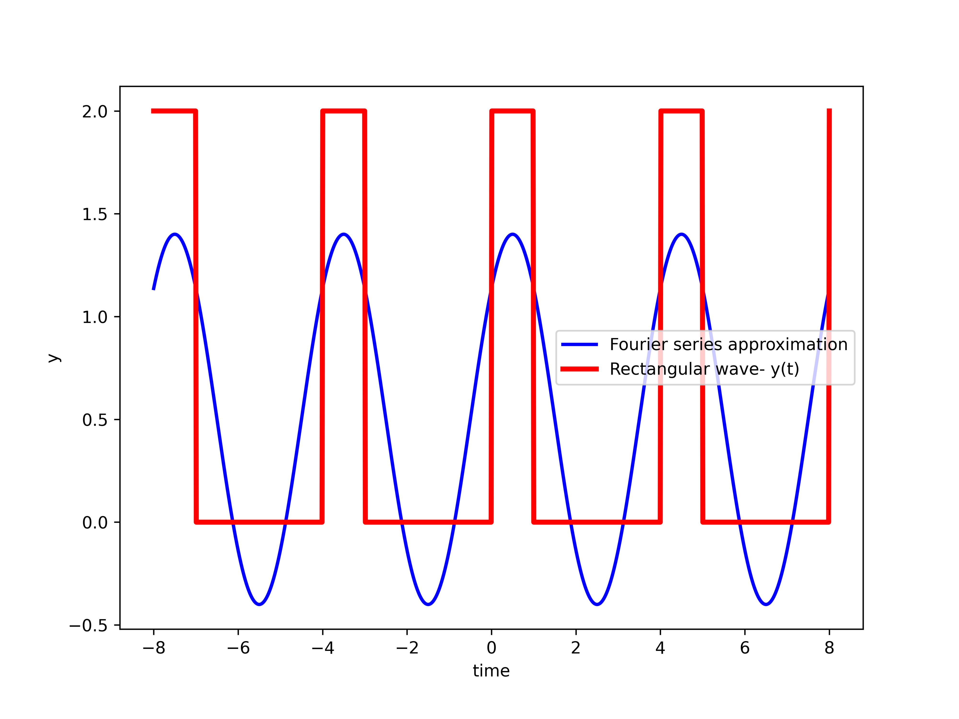Figure 2: Approximation of the rectangular wave (red) by using Fourier series (blue). The approximation is obtained for $k=0,\pm 1$ , and is given by (11).

For $k=0,\pm 1, \pm 2, \pm 3$ , we obtain the following approximation

(12) $\begin{align*}& - 0.31831 i e^{i \pi t} + \left(0.31831 - 0.31831 i\right) e^{\frac{i \pi t}{2}} + 0.5 \\& + \left(0.31831 + 0.31831 i\right) e^{- \frac{i \pi t}{2}}+ 0.31831 i e^{- i \pi t}\end{align*}$

The approximation is shown below.

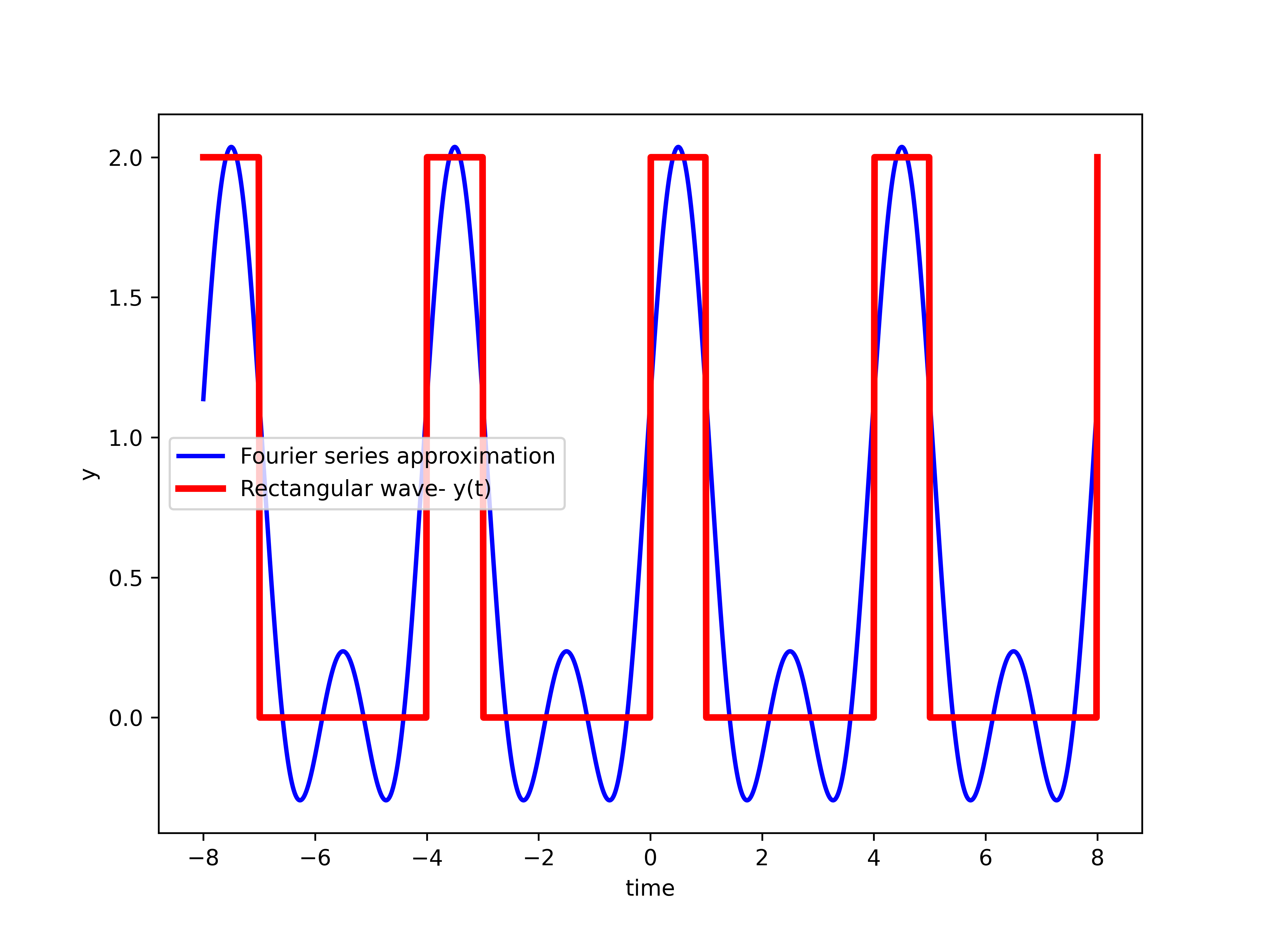
Figure 3: Approximation of the rectangular wave (red) by using Fourier series (blue). The approximation is obtained for $k=0,\pm 1,\pm 2$ , and is given by (12).

For $k=0,\pm 1,\pm 2,\ldots , \pm 10$ , the approximation is shown in the figure below.

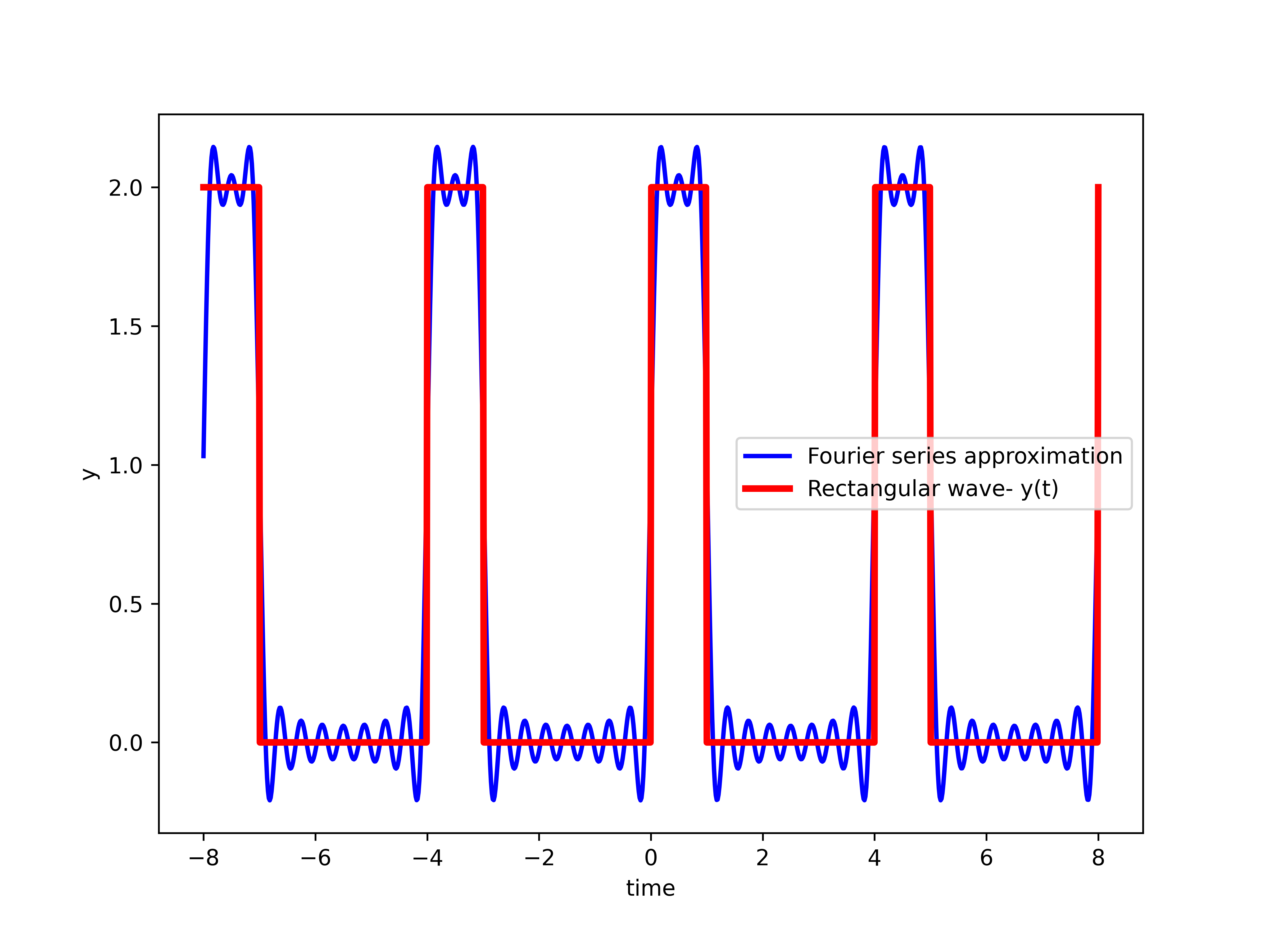
Figure 4: Approximation of the rectangular wave (red) by using Fourier series (blue). The approximation is obtained for $k=0,\pm 1,\pm 2,\ldots, \pm 10$ .

Example 1: Finite Fourier Series

We consider the following example

(13) $\begin{align*}y(t)=2+\cos(\omega_{0}t)+\sin(2\omega_{0}t)+\cos(2\omega_{0}t+\frac{\pi}{3})\end{align*}$

The goal is to compute the Fourier series expansion of this function.

For $T_{0}=0.5$ , the function is illustrated in the figure below.

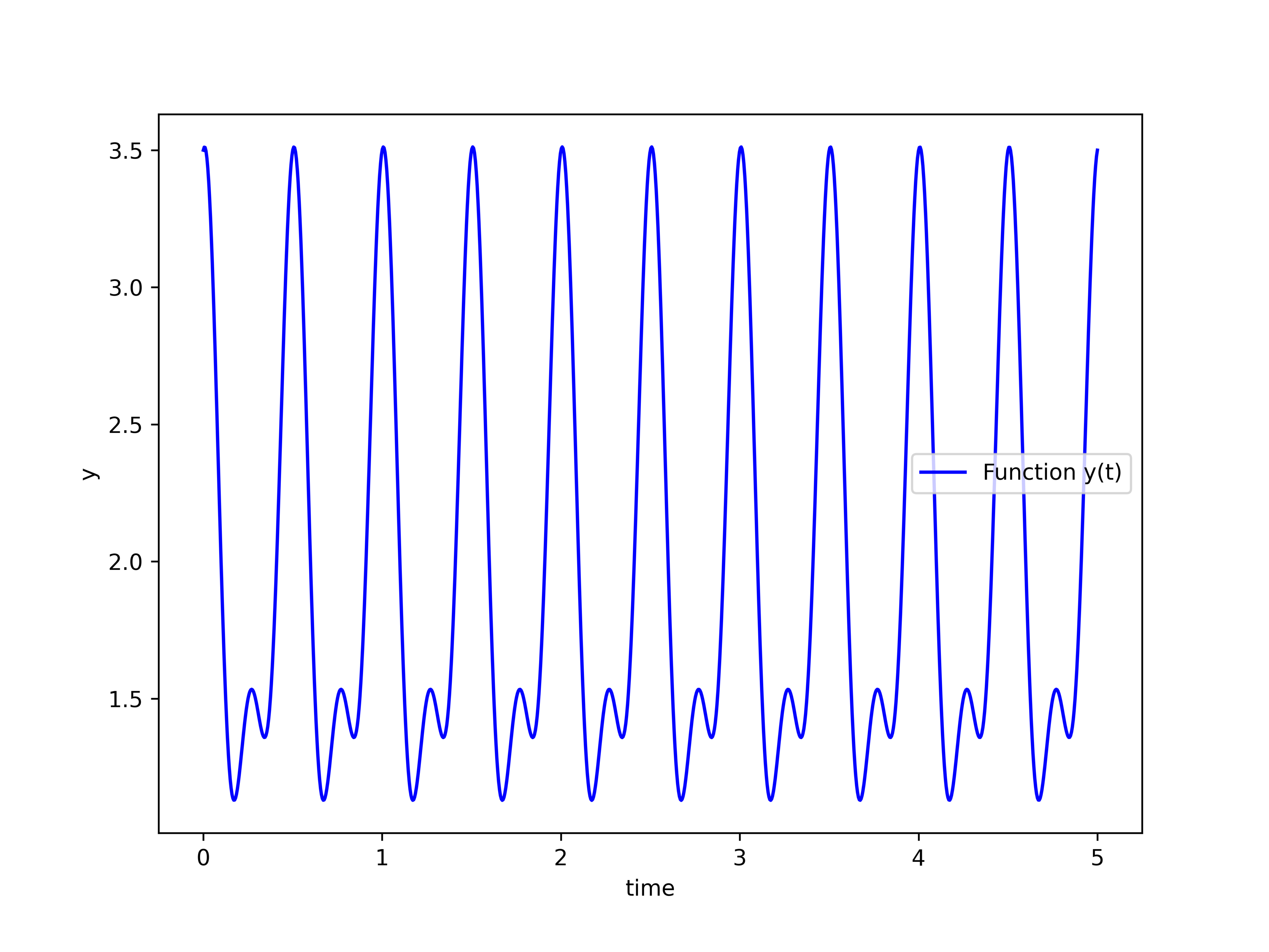
Figure 2: Function (13) obtained for $T_{0}=0.5$

The following Python script is used to generate this graph.

import numpy as np
import matplotlib.pyplot as plt

To=0.5
omega0=2*np.pi/To

timeVector=np.linspace(0,5,1000)

y=2+np.cos(omega0*timeVector)+np.sin(2*omega0*timeVector)+np.cos(2*omega0*timeVector+np.pi/3)


# plot the results 
plt.figure(figsize=(8,6))
plt.plot(timeVector, y,'b',label='Function y(t)')
plt.xlabel('time')
plt.ylabel('y')
plt.legend()
plt.savefig('originalFunction.png',dpi=600)
plt.show()

There are two approaches for computing the Fourier series coefficients. The first approach is to use the formula (4). As we will show in the next example, this involves significant effort. However, since this function is a sum of harmonic functions ( $\sin$ and $\cos$ functions), there is a direct and less time-consuming approach for calculating the Fourier series. Namely, we can use the following formulas

(14) $\begin{align*}\sin (\theta)=\frac{e^{j\theta}-e^{-j\theta}}{2j} \\\cos (\theta) = \frac{e^{j\theta}+e^{-j\theta}}{2}\end{align*}$

where $\theta$ is an argument or an angle of $\sin ()$ or $\cos ()$ function. By substituting every harmonic function in (13), by its exponential form (14), we have

(15) $\begin{align*}y(t)=& \underbrace{2e^{j0\omega_{0}t}}_{2} \\ & + \underbrace{\frac{e^{j\omega_{0}t}+e^{-j\omega_{0}t}}{2}}_{\cos(\omega_{0}t)} +\underbrace{\frac{e^{j2\omega_{0}t}-e^{-j2\omega_{0}t}}{2j}}_{\sin(2\omega_{0}t)} \\& + \underbrace{\frac{e^{j(2\omega_{0}t+\frac{\pi}{3})}+e^{-j(2\omega_{0}t+\frac{\pi}{3})}}{2} }_{\cos(2\omega_{0}t+\frac{\pi}{3})}\end{align*}$

The last equation can be written as follows

(16) $\begin{align*}y(t) & =2e^{j0\omega_{0}t}+\frac{1}{2}e^{j\omega_{0}t}+\frac{1}{2}e^{-j\omega_{0}t} \\& +\big(\frac{1}{2j}+\frac{1}{2}e^{j\frac{\pi}{3}} \big)e^{j2\omega_{0}t}+\big(\frac{1}{2}e^{-j\frac{\pi}{3}}-\frac{1}{2j} \big) e^{-j2\omega_{0}t}\end{align*}$

or in the required Fourier series expansion form

(17) $\begin{align*}y(t)=c_{0}e^{j0\omega_{0}t}+c_{1}e^{j\omega_{0}t}+c_{-1}e^{-j\omega_{0}t}+c_{2} e^{j2\omega_{0}t}+c_{-2} e^{-j2\omega_{0}t}\end{align*}$

where the Fourier series coefficients are

(18) $\begin{align*}c_{0}& =2 \\c_{1}& = \frac{1}{2} \\c_{-1}& = \frac{1}{2} \\c_{2} & = \frac{1}{2j}+\frac{1}{2}e^{j\frac{\pi}{3}} =-\frac{1}{2}j+\frac{1}{2}e^{j\frac{\pi}{3}} \\c_{-2} & = \frac{1}{2}e^{-j\frac{\pi}{3}}-\frac{1}{2j} = \frac{1}{2}j+\frac{1}{2}e^{-j\frac{\pi}{3}}\end{align*}$

We can also verify that these are correct coefficients by using the following Python script. The Python script given below will be thoroughly explained in out future tutorials.

from sympy import *
t = Symbol('t', real=True)
To=0.5
omega0=2*pi/To

y=2+cos(omega0*t)+sin(2*omega0*t)+cos(2*omega0*t+pi/3)
coeffNumber=[-2, -1, 0, 1, 2]
computedCoefficients=[]


for coeff in coeffNumber:
    answer=((1/To)*integrate(y*exp((-coeff*I*omega0*t)),(t, 0, To))).simplify().evalf(6)
    computedCoefficients.append(answer)    

# double check, the coefficients c2 and c_{-2}
# compare these coefficients with the ones in computedCoefficients
c_2=(-0.5*I+0.5*E**(I*pi/3)).simplify().evalf(6)
c_m2=(0.5*I+0.5*E**(-I*pi/3)).simplify().evalf(6)

Example 2: Infinite Fourier Series of Periodic Rectangular Wave (Periodic Pulse Function)

We want to compute the Fourier series expansion of the periodic rectangular wave function shown below.

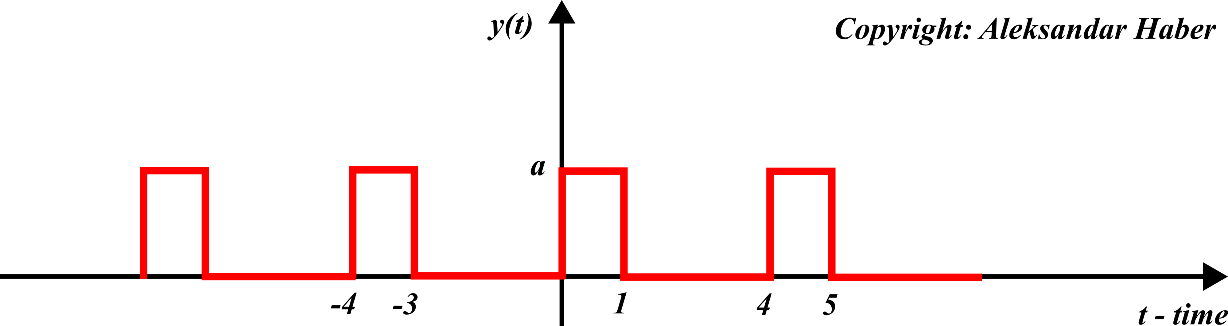
Figure 3: Periodic rectangular wave function.

The amplitude of the wave is equal to $a$ . The first step is to identify the fundamental period $T_{0}$ . We can see that this function repeats itself every $4$ seconds. Consequently, we have $T_{0}=4$ .

To compute the Fourier series expansion we need to compute the following integral:

(19) $\begin{align*}c_{k}=\frac{1}{T_{0}}\int_{0}^{T_{0}}y(t)e^{-jk\omega_{0}t} \mathrm{d}t\end{align*}$

Taking into account the shape of the function $y(t)$ shown in Fig. 3, we have

(20) $\begin{align*}c_{k} & =\frac{1}{T_{0}}\int_{0}^{T_{0}}y(t)e^{-jk\omega_{0}t} \mathrm{d}t= \frac{1}{4}\int_{0}^{4}y(t)e^{-jk\omega_{0}t} \mathrm{d}t \\& = \frac{1}{4}\Big( \int_{0}^{1}a\cdot e^{-jk\omega_{0}t} \mathrm{d}t + \int_{1}^{4} 0\cdot e^{-jk\omega_{0}t} \mathrm{d}t \Big) \\& = \frac{1}{4} \int_{0}^{1}a\cdot e^{-jk\omega_{0}t} \mathrm{d}t = \frac{a}{4} \int_{0}^{1} e^{-jk\omega_{0}t} \mathrm{d}t \\& =\frac{a}{4}\cdot \frac{e^{-jk\omega_{0}t} }{-jk\omega_{0}}\Bigg|_{0}^{1} \\& = \frac{a}{-j(4k\omega_{0})}\Big(e^{-jk\omega_{0}} -1 \Big) \\& =\frac{a}{-j(4k\omega_{0})} e^{-j\frac{k\omega_{0}}{2}}\Big(e^{-j\frac{k\omega_{0}}{2}} -e^{j\frac{k\omega_{0}}{2}} \Big)\\& =\frac{a}{j(4k\omega_{0})} e^{-j\frac{k\omega_{0}}{2}}\Big(e^{j\frac{k\omega_{0}}{2}}-e^{-j\frac{k\omega_{0}}{2}} \Big)\\& =\frac{a}{2k\omega_{0}} e^{-j\frac{k\omega_{0}}{2}} \cdot \frac{e^{j\frac{k\omega_{0}}{2}}-e^{-j\frac{k\omega_{0}}{2}}}{2j} \\& =\frac{a}{2k\omega_{0}} e^{-j\frac{k\omega_{0}}{2}} \sin \big( \frac{k\omega_{0}}{2} \big)\end{align*}$

By substituting

(21) $\begin{align*}\omega_{0}=\frac{2\pi}{T_{0}}=\frac{2\pi}{4}=\frac{\pi}{2}\end{align*}$

in the last equation of (20), we have

(22) $\begin{align*}c_{k} = \frac{a}{2k\frac{\pi}{2}} e^{-j\frac{k\frac{\pi}{2}}{2}} \sin \big( \frac{k\frac{\pi}{2}}{2} \big)\end{align*}$

(23) $\begin{align*}c_{k} = \frac{a}{k\pi} e^{-j\frac{k\pi}{4}} \sin \big( \frac{k\pi}{4} \big)\end{align*}$

This is the final expression of the Fourier coefficient. We can also write this expression like this

(24) $\begin{align*}c_{k} = \frac{a}{4}\cdot e^{-j\frac{k\pi}{4}} \cdot \frac{\sin \big( \frac{k\pi}{4} \big)}{\frac{k\pi}{4}}\end{align*}$

We need to explicitly compute $c_{0}$ :

(25) $\begin{align*}c_{0}=\lim_{k \rightarrow 0} \frac{a}{4}\cdot e^{-j\frac{k\pi}{4}} \cdot \frac{\sin \big( \frac{k\pi}{4} \big)}{\frac{k\pi}{4}} =\frac{a}{4}\end{align*}$

This is because

(26) $\begin{align*}\lim_{k \rightarrow 0} \frac{\sin \big( \frac{k\pi}{4} \big)}{\frac{k\pi}{4}} =1\end{align*}$

We can use the following Python script to compute and verify the solution

from sympy import *
t = Symbol('t', real=True)
To=4
omega0=2*pi/To
a=2

# derived formula
k=3

c=(a/(k*pi))*sin(k*pi/4)*E**(-I*k*pi/4)
c=c.simplify().evalf(6)

# use the definition
computedIntegral=((1/To)*integrate(a*exp((-k*I*omega0*t)),(t, 0, 1))).simplify().evalf(6)

Basics of Fourier Series and Main Formulas

Example 1: Finite Fourier Series

Example 2: Infinite Fourier Series of Periodic Rectangular Wave (Periodic Pulse Function)

admin

You might also like

Control Systems Lecture: Laplace Transform

Automatic State-Space Derivation and Simulation of Nonlinear Dynamical Systems in Python with Inverted Pendulum on a Cart Example

Design and Test Observers of Dynamical Systems in MATLAB