Automatically Compute Jacobians of Vector Functions in Python by Using Symbolic Library – Fusion of Engineering, Control, Coding, Machine Learning, and Science

In this Python scientific computing, signal processing, optimization, and control theory tutorial you will learn how to automatically compute Jacobians of vector functions in Python by using the symbolic Python library called SymPy. Furthermore, you will learn how to automatically generate code that will return the Jacobian matrix for the specified input vector. That is, you will learn how to write a Python script that will evaluate the value of the Jacobian matrix for the specified input vector (point in $n$ -dimensional space). This tutorial is very important for engineers and students who want to develop optimization solvers or signal processing and control engineering algorithms in Python. Namely, a number of optimization solvers and control engineering algorithms are based on the computation of the Jacobians of nonlinear functions.

Here is a brief summary of the video tutorial. First, we provide a brief summary of Jacobian matrices of vector functions. We briefly introduce vector functions and explain how to compute Jacobian matrices of vector functions. Then, in order to test our Python implementation, we construct an example of a nonlinear vector function. We explain how to analytically compute the Jacobian matrix of this function. The computed analytical form of the Jacobian is used to test our Python implementation. Finally, we explain how to compute the Jacobian matrices in Python by using the SymPy library and how to generate Python functions out of computed symbolic expressions.

The YouTube video accompanying this webpage tutorial is given below.

Brief Summary of Jacobians of Vector Functions

Before we explain how to write Python scripts, we first need to briefly summarize the concept of Jacobian matrices. Consider the following vector function that takes as an input the $n$ -dimensional vector $\mathbf{x}\in \mathbb{R}^{n}$ and it maps this vector into the $m$ -dimensional vector:

(1) $\begin{align*}\mathbf{f}(\mathbf{x})=\begin{bmatrix} f_{1}(x_{1},x_{2},x_{3},\ldots, x_{n}) \\ f_{2}(x_{1},x_{2},x_{3},\ldots, x_{n}) \\ \vdots \\ f_{m}(x_{1},x_{2},x_{3},\ldots, x_{n}) \end{bmatrix}\end{align*}$

where the vector $\mathbf{x}$ is defined by

(2) $\begin{align*}\mathbf{x}=\begin{bmatrix}x_{1} \\ x_{2} \\ \vdots \\ x_{n} \end{bmatrix}\end{align*}$

The nonlinear vector function $\mathbf{f}$ produces the $m$ -dimensional vector

(3) $\begin{align*}\begin{bmatrix} f_{1}(x_{1},x_{2},x_{3},\ldots, x_{n}) \\ f_{2}(x_{1},x_{2},x_{3},\ldots, x_{n}) \\ \vdots \\ f_{m}(x_{1},x_{2},x_{3},\ldots, x_{n}) \end{bmatrix}\end{align*}$

whose entries are $m$ functions $f_{i}$ , $i=1,2,\ldots, n$ that map the entries of the vector $\mathbf{x}$ into scalar numbers.

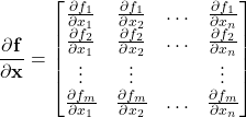
The Jacobian matrix of the function $\mathbf{f}(\cdot )$ is $m$ by $n$ dimensional matrix of partial derivatives defined by

(4) $\begin{align*}\frac{\partial \mathbf{f} }{\partial \mathbf{x}}=\begin{bmatrix} \frac{\partial f_{1}}{\partial x_{1}} & \frac{\partial f_{1}}{\partial x_{2}} & \ldots & \frac{\partial f_{1}}{\partial x_{n}} \\ \frac{\partial f_{2}}{\partial x_{1}} & \frac{\partial f_{2}}{\partial x_{2}} & \ldots & \frac{\partial f_{2}}{\partial x_{n}} \\ \vdots & \vdots & & \vdots \\ \frac{\partial f_{m}}{\partial x_{1}} & \frac{\partial f_{m}}{\partial x_{2}} & \ldots & \frac{\partial f_{m}}{\partial x_{n}} \end{bmatrix}\end{align*}$

The first row of this matrix consists of partial derivatives of $f_{1}(\cdot)$ with respect to $x_{1},x_{2},\ldots, x_{n}$ , respectively. Similarly, the second row of this matrix consists of partial derivatives of $f_{2}(\cdot)$ with respect to $x_{1},x_{2},\ldots, x_{n}$ , respectively. In the same manner, we construct the other rows of the Jacobian matrix.

Python Script for Symbolically Computing the Jacobian Matrix

Here, we present the Python script for symbolically computing the Jacobian matrix and for creating the Python function that will return the numerical values of the Jacobian matrix for the given input vector $\mathbf{x}$ . To verify the Python implementation, let us consider the following test-case function

(5) $\begin{align*}\mathbf{f}=\begin{bmatrix} x_{1}x_{2} \\ \sin(x_{1}) \\ \cos(x_{3}) \\ x_{3}e^{x_{4}} \end{bmatrix}\end{align*}$

where $\mathbf{x}$ is

(6) $\begin{align*}\mathbf{x}=\begin{bmatrix}x_{1}\\ x_{2} \\ x_{3} \\ x_{4} \end{bmatrix}\end{align*}$

and

(7) $\begin{align*}f_{1}(x_{1},x_{2},x_{3},x_{4}) & =x_{1}x_{2} \\f_{2}(x_{1},x_{2},x_{3},x_{4}) & = \sin(x_{1}) \\f_{3}(x_{1},x_{2},x_{3},x_{4}) & = \cos(x_{3}) \\f_{4}(x_{1},x_{2},x_{3},x_{4}) & = x_{3}e^{x_{4}} \end{align*}$

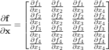
The Jacobian of this function is

(8) $\begin{align*}\frac{\partial \mathbf{f} }{\partial \mathbf{x}}=\begin{bmatrix} \frac{\partial f_{1}}{\partial x_{1}} & \frac{\partial f_{1}}{\partial x_{2}} & \frac{\partial f_{1}}{\partial x_{3}} & \frac{\partial f_{1}}{\partial x_{4}} \\ \frac{\partial f_{2}}{\partial x_{1}} & \frac{\partial f_{2}}{\partial x_{2}} & \frac{\partial f_{2}}{\partial x_{3}} & \frac{\partial f_{2}}{\partial x_{4}} \\ \frac{\partial f_{3}}{\partial x_{1}} & \frac{\partial f_{3}}{\partial x_{2}} & \frac{\partial f_{3}}{\partial x_{3}} & \frac{\partial f_{3}}{\partial x_{4}} \\ \frac{\partial f_{4}}{\partial x_{1}} & \frac{\partial f_{4}}{\partial x_{2}} & \frac{\partial f_{4}}{\partial x_{3}} & \frac{\partial f_{4}}{\partial x_{4}} \end{bmatrix}\end{align*}$

By computing these partial derivatives, we obtain

(9) $\begin{align*}\frac{\partial \mathbf{f} }{\partial \mathbf{x}}= \begin{bmatrix} x_{2} & x_{1} & 0 & 0 \\ \cos(x_{1}) & 0 & 0 & 0 \\ 0 & 0 & -\sin(x_{3}) & 0 \\ 0 & 0 & e^{x_{4}} & x_{3}e^{x_{4}} \end{bmatrix}\end{align*}$

The Python script shown below is used to symbolically compute the Jacobian matrix and to generate a Python function that returns the numerical values of the Jacobian matrix.

# import the necessary libraries
import numpy as np
# sympy library - we import everything
from sympy import *
# this function is used to generate nice 
# prints of symbolic expressions
init_printing()

# define the symbolic vector x
x=MatrixSymbol('x',4,1)

# here, we define our function f as 4 by 1 matrix 
f=Matrix([[x[0]*x[1]],
          [sin(x[0])],
          [cos(x[2])],
          [x[2]*E**(x[3])]])

# here, we symbolically compute the Jacobian matrix
JacobianSymbolic=f.jacobian(x)

# here, we create a Python function that returns the 
# numerical value of the Jacobian
JacobianFunction=lambdify(x,JacobianSymbolic)

# we create a test case vector
testCaseVector=np.array([[1],[1],[1],[1]])

# here, we evaluate the numerical value of the Jacobian matrix
JacobianNumerical=JacobianFunction(testCaseVector)

We define the symbolic vector “x” for our computation as follows

# define the symbolic vector x
x=MatrixSymbol('x',4,1)

The nonlinear vector function “f” is defined by

=Matrix([[x[0]*x[1]],
          [sin(x[0])],
          [cos(x[2])],
          [x[2]*E**(x[3])]])

Here, it should be kept in mind that the SymPy library uses “E” to denote the exponential function $e$ . We use the following code line to compute the Jacobian matrix

# here, we symbolically compute the Jacobian matrix
JacobianSymbolic=f.jacobian(x)

Then, we create a Python function out of the return symbolic matrix as follows

# numerical value of the Jacobian
JacobianFunction=lambdify(x,JacobianSymbolic)

To do that, we use the SymPy function “lambdify”. This function is used to create Python functions out of symbolic expressions. The first argument of this function is the symbolic variable, and the second argument is the symbolic expression.

Finally, we evaluate the Jacobian at a test vector.

# we create a test case vector
testCaseVector=np.array([[1],[1],[1],[1]])

# here, we evaluate the numerical value of the Jacobian matrix
JacobianNumerical=JacobianFunction(testCaseVector)

The result that is stored in “JacobianNumerical” is a NumPy array (matrix) of numerical values that can be used to further computations.

Brief Summary of Jacobians of Vector Functions

Python Script for Symbolically Computing the Jacobian Matrix

admin

You might also like

Homework Assignment 3

Review of Torsion

Forward Robot Kinematics Using Homogeneous Transform