 by
by
In this tutorial, we explain how to simulate ordinary differential equations in Simulink. The YouTube tutorial accompanying this webpage is given below.
Example and Preparation Steps
We explain the simulation process by using a particular example.
Problem: Simulate ordinary differential equation
(1) 
where  is a dependent variable (that we want to solve for),
  and
and  are real constants, and
  is an external real input. In (1), the “dot” symbol above the dependent variable denotes the first derivative. To make the problem numerically tractable, we assume the following values
  ,
,  , and
, and  .
.
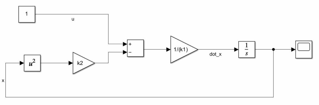
The Simulink model is shown in the figure below.
The simulated solution is shown in the figure below.
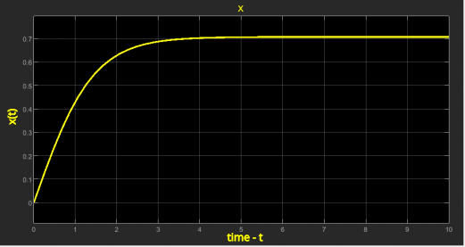
 .
.In the sequel, we explain how to create this model.
Before we start with the Simulink modeling, we first need to transform our equation into the appropriate form. The transformation process consists of the following steps.
STEP 1: In this step, we want to express the first derivative of . That is, on the left-hand side of the equation (1), we only need to have  :
:
(2) 
STEP 2: In this step, we eliminate the first derivative by using the fact that the first derivative of is equivalent to the product of  and
and  in the Laplace complex domain, where is the complex variable. That is,
  . Here, not to make the notation too complex, we will simply denote the Laplace transformation of the time domain variable , by . The product of and is interpreted as the derivative of . Later on, we will interpret the product of
  and as an integral of . We obtain
(3) 
STEP 3: Similarly to STEP 1, we move the variable from the left to the right-hand side of the last equation. That is, on the left-hand side of the equation we need only to have :
(4) 
The term
(5) 
is an integrator. It is modeled as an integrator block in Simulink.
Now, we are ready to construct the Simulink block diagram.
Simulink Implementation
First, we create a new MATLAB script and define the variables
(6) 
We load these variables in the MATLAB workspace. The Simulink workspace is able to directly read these variables from the MATLAB workspace.
Next, we construct the expression in the brackets
(7) 
The Simulink block diagram is shown below.
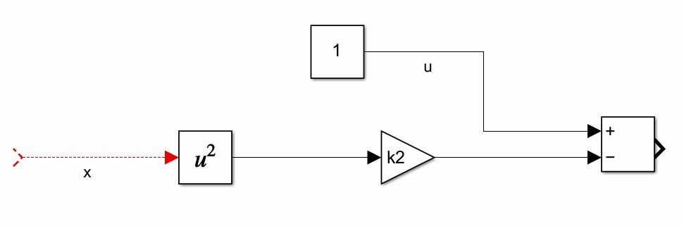
 .
. Next, we include the constant  and the integrator . The Block diagram is shown below
 and the integrator .
Finally, we add the feedback and the scope. This is shown in the figure below.
