Influence of Zeros and Non-Minimum Phase Zeros of Transfer Functions on Dynamical System Behavior – Fusion of Engineering, Control, Coding, Machine Learning, and Science

In this tutorial, we cover one very important topic that is often overlooked in control engineering university courses. We explain the effect of zeros of transfer functions on dynamical system behavior. A proper understanding of the zeros of dynamical systems is very important for properly designing feedback control systems. The YouTube video tutorial accompanying this tutorial is given below. This tutorial is partly based on the material presented in Chapter 3.5 of Feedback Control of Dynamic Systems (third edition), by Franklin, Powell, and Emami-Naeini and on the basis of the material presented in Modern Control Engineering by K. Ogata.

Zero close to the real pole attenuates the effect of that pole on the system response

Let us consider the following transfer function

(1) $\begin{align*}W_{1}(s)=\frac{4}{(s+1)(s+4)}\end{align*}$

The impulse response of this system can be computed by computing the partial fraction expansion. The partial fractional expansion is given by

(2) $\begin{align*}W_{1}=\frac{C_{1}}{s+1}+\frac{C_{2}}{s+4}\end{align*}$

We compute the coefficients $C_{1}$ and $C_{2}$ by using the cover method

(3) $\begin{align*}C_{1}=W_{1}(s+1)\vert_{s=-1}=\frac{4}{3} \\C_{2}=W_{1}(s+4)\vert_{s=-4}=-\frac{4}{3}\end{align*}$

Consequently, we have

(4) $\begin{align*}W_{1}=\frac{4}{3}\cdot \frac{1}{s+1}-\frac{4}{3}\cdot\frac{1}{s+4}\end{align*}$

The impulse response in the time domain is given by the inverse Laplace transform of $W_{1}$ :

(5) $\begin{align*}y_{1}(t)=\frac{4}{3}e^{-t}-\frac{4}{3}e^{-4t}\end{align*}$

Later on, we will plot this response in MATLAB. Next, let us modify the transfer function by including a zero close to the pole, and let us scale the new transfer function such that it has the same steady-state gain as the steady-state gain of the original transfer function. Let the modified transfer function be given by

(6) $\begin{align*}W_{2}=\frac{4(s+0.9)}{0.9(s+1)(s+4)}\end{align*}$

where $s=-0.9$ is a zero very close to the pole $s=-1$ The partial fraction expansion of this transfer function is given by

(7) $\begin{align*}W_{2}=\frac{C_{1}}{s+1}+\frac{C_{2}}{s+4}=-0.1481\cdot \frac{1}{s+1}+4.5926\cdot \frac{1}{s+4}\end{align*}$

where $C_{1}=-0.1481$ and $C_{2}=4.5926$ . We can immediately see that the zero $s=-0.9$ close to the pole $s=-1$ significantly diminishes the value of the coefficient $C_{1}$ . This comes from the fact that

(8) $\begin{align*}C_{1}=W_{2}(s+1)\vert_{s=-1}=\text{small number due to the term}\;\; s+0.9\end{align*}$

That is, a zero close to a pole decreases the effect of that pole on the response of the system. The impulse response of the system $W_{2}$ is given by

(9) $\begin{align*}y_{2}(t)=-0.1481e^{-t}+4.5926e^{-4t}\end{align*}$

Let us now plot the impulse responses of the two systems. We use the MATLAB code shown below to plot the impulse response.

clear
s=tf('s')
W1=4/((s+1)*(s+4))
figure (1)
hold on
impulse(W1,'r')
W2=(4*(s+0.9))/(0.9*(s+1)*(s+4))
impulse(W2,'k')

The impulse response is shown in the figure below.

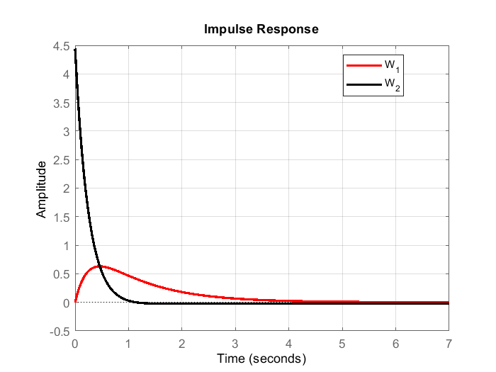Figure 1: Impulse responses of the system without zeros ( $W_{1}$ ) and with zeros ( $W_{2}$ ).

The red line represents the impulse response of the system $W_{1}$ that does not contain zeros. The black line is the impulse response of the system with the zero close to the pole. However, we can observe that the impulse response of the system $W_{2}$ initially has a large value. This is mainly due to the derivative action interpretation of additional zeros. This will be explained in the sequel.

Zeros Tend to Increase the Overshoot of the System

Next, we explain another phenomenon caused by zeros. Namely, under certain circumstances, the zeros tend to increase the overshoot of the system’s step response. Let us explain this important phenomenon by considering a prototype second-order system given by the following equation:

(10) $\begin{align*}W=\frac{\omega_{n}^{2}}{s^{2}+2\zeta \omega_{n}s+\omega_{n}^{2}}\end{align*}$

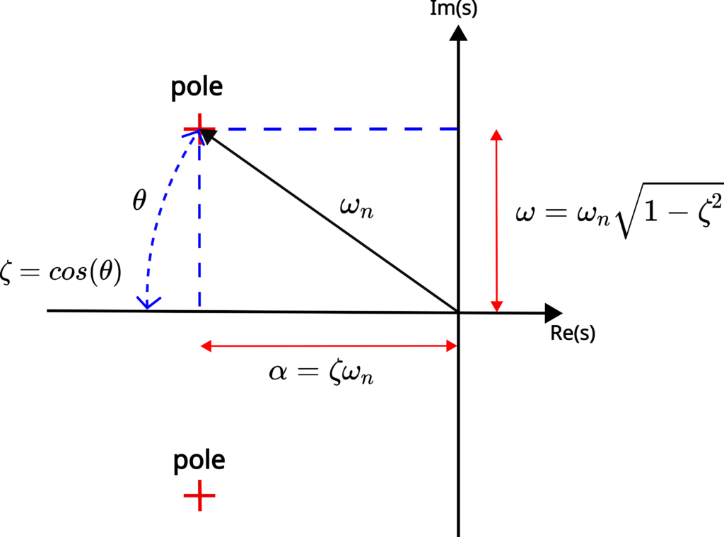
where $\omega_{n}$ is the natural undamped frequency and $\zeta$ is the damping ratio. We explained the motivation for introducing this prototypical system in our previous tutorial which can be found here. The poles of this system are given by

(11) $\begin{align*}s_{1,2}=-\zeta \omega_{n}\pm \omega_{n}\sqrt{1-\zeta^2}j\end{align*}$

These poles are illustrated in the figure below.

Figure 2: Poles of the prototype system.

The system (10) can be transformed as follows

(12) $\begin{align*}W=\frac{\omega_{n}^{2}}{s^{2}+2\zeta \omega_{n}s+\omega_{n}^{2}}=\frac{1}{(\frac{s}{\omega_{n}})^2+2\zeta (\frac{s}{\omega_{n}})+1} \end{align*}$

Next, let us add a zero term to the prototype system

(13) $\begin{align*}\frac{s}{k\zeta \omega_{n}}+1\end{align*}$

The zero is given by

(14) $\begin{align*}s=-k\zeta \omega_{n}\end{align*}$

where $k$ is the parameter that we will vary. The final transfer function is given by

(15) $\begin{align*}W_{F}=\frac{\frac{s}{k\zeta \omega_{n}}+1}{(\frac{s}{\omega_{n}})^2+2\zeta (\frac{s}{\omega_{n}})+1} \end{align*}$

Since the real part of the poles is $-\zeta \omega_{n}$ , for $k=1$ , the zero given in (14) will precisely be at the location of the real part of the pole. Next, we simulate the step response of the system (15) for several values of $k$ . The results are shown in the figure below.

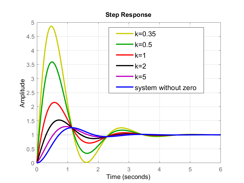
The blue line in the figure above shows the step response of the system (12) without the zero. On the other hand, lines with other colors show the responses of the system (15) with the zero given by (14). We can observe that the overshoot of the system is significantly increased compared to the system without the zero. As $k$ is increased, the zero (14) is moved further away from the real part of the pole. That is, as $k$ is increased, the zero is moved further to the left in the complex plane. As the zero is moved away from the real part of the poles, the overshoot is decreased. On the other hand, as $k$ is decreased, the zero becomes closer and closer to the real part of the pole and the imaginary axis. For $k=1$ , the zero is precisely at the location of the real part of the pole. The overshoot gets larger and larger as $k$ becomes smaller and smaller. Also, we can observe that the introduced zero has almost no effect on the settling time. As k is decreased, that is, as zero approaches the imaginary axis the rise time of the system is decreased. The MATLAB code used to generate Fig. 3 is given below.

clear,clc
zeta=0.4
omega_n=3

s=tf('s')

k=0.35
Wm1=((s/(k*zeta*omega_n))+1)/((s/omega_n)^2+2*zeta*(s/omega_n)+1)
 
figure(1)
hold on 
step(Wm1,'y')


k=0.5
W0=((s/(k*zeta*omega_n))+1)/((s/omega_n)^2+2*zeta*(s/omega_n)+1)
 
figure(1)
hold on 
step(W0,'g')


k=1
W1=((s/(k*zeta*omega_n))+1)/((s/omega_n)^2+2*zeta*(s/omega_n)+1)
 
figure(1)
hold on 
step(W1,'r')
 
k=2
W2=((s/(k*zeta*omega_n))+1)/((s/omega_n)^2+2*zeta*(s/omega_n)+1)
hold on 
step(W2,'k')
 
k=5
W3=((s/(k*zeta*omega_n))+1)/((s/omega_n)^2+2*zeta*(s/omega_n)+1)
hold on 
step(W3,'m')
 
W4=1/((s/omega_n)^2+2*zeta*(s/omega_n)+1)
hold on 
step(W4,'b')

Next, we explain the reason for the increase of overshoot. Let us make the following substitution

(16) $\begin{align*}v=\frac{s}{\omega_{n}}\end{align*}$

where $v$ is a new scaled complex variable. In the time domain, this substitution corresponds to the scaling of time. By substituting (16) in (15), we obtain

(17) $\begin{align*}W_{F}=\frac{\frac{v}{k\zeta}+1}{v^2+2\zeta v+1} \end{align*}$

where $v$ is now a new complex Laplace variable. We can expand this function as follows:

(18) $\begin{align*}W_{F}=\frac{1}{v^2+2\zeta v+1} +\frac{1}{k\zeta}\cdot \frac{v}{v^2+2\zeta v+1} \end{align*}$

Next, let us define the following transfer functions

(19) $\begin{align*}W_{F1}=\frac{1}{v^2+2\zeta v+1},\;\; W_{F2}=\frac{v}{v^2+2\zeta v+1} \end{align*}$

That is, we have

(20) $\begin{align*}W_{F}=W_{F1}+\frac{1}{k\zeta} W_{F2}=\frac{1}{v^2+2\zeta v+1} +\frac{1}{k\zeta}\cdot \frac{v}{v^2+2\zeta v+1} \end{align*}$

It should be observed that

(21) $\begin{align*}W_{F2}=v\cdot W_{F1}\end{align*}$

Our task is to first compute the impulse response of $W_{F}$ . The impulse response is

(22) $\begin{align*}y_{i}(\tau )=\mathcal{L}^{-1}\left\{ W_{F} \right\}=\mathcal{L}^{-1}\left\{ W_{F1} \right\}+\mathcal{L}^{-1}\left\{ \frac{1}{k\zeta} W_{F2} \right\}\end{align*}$

where $\mathcal{L}^{-1}\left\{ \cdot \}$ is the inverse Laplace transform operator, and $\tau$ is a scaled time induced by the transformation (16). Now, let us introduce this notation

(23) $\begin{align*}y_{i1}(\tau )=\mathcal{L}^{-1}\left\{ W_{F1} \right\} \\y_{i2}(\tau )=\mathcal{L}^{-1}\left\{ \frac{1}{k\zeta} W_{F2} \right\}=\frac{1}{k\zeta}\mathcal{L}^{-1}\left\{ W_{F2} \right\}\end{align*}$

By using this new notation, we can write

(24) $\begin{align*}y_{i}(\tau )=\mathcal{L}^{-1}\left\{ W_{F} \right\}= y_{i1}(\tau )+y_{i2}(\tau )\end{align*}$

It is a very well-known fact that the Laplace transform of the first derivative of a function is actually $s$ times the Laplace transform of the function (if we ignore the initial conditions). For example, if $f(t)$ is a time domain function, and if $F(s)$ is its Laplace transform, then we have

(25) $\begin{align*}\mathcal{L}\left\{ \dot{f}(t) \right \}=sF(s)\end{align*}$

In our case, we have a scaled complex variable $v$ . Then, from (21), it follows that

(26) $\begin{align*}\mathcal{L}^{-1}\left\{ W_{F2} \right\}=\mathcal{L}^{-1}\left\{ v\cdot W_{F1} \right\}=\dot{y}_{i1}(\tau )\end{align*}$

where $y_{i1}$ is the inverse Laplace transform of $W_{F1}$ . Consequently, the second term in (24) can be interpreted as the first derivative of $y_{i1}$ multiplied by a constant $1/(k \zeta )$ . That is, we can write (24) as follows

(27) $\begin{align*}y_{i}(\tau )=y_{i1}(\tau )+\frac{1}{k \zeta }\dot{y}_{i1}(\tau )\end{align*}$

From this analysis, we conclude that the zeros introduce a derivative action during the initial part of the transient response. This analysis can also be applied to the step response of the system simply because the step response in the complex domain is given by

(28) $\begin{align*}Y(v) & =W_{F}U(v)=W_{F}\frac{1}{v} \\Y(v) & =W_{F1}\frac{1}{v}+\frac{1}{k\zeta}\cdot W_{F2}\frac{1}{v} \\Y(v) & = \frac{1}{v^2+2\zeta v+1}\cdot \frac{1}{v}+\frac{1}{k\zeta}\cdot \frac{v}{v^2+2\zeta v+1} \frac{1}{v} \\Y(v) & =\underbrace{W_{F1}\cdot \frac{1}{v}}_{W_{F1}^{\text{new}}}+\frac{1}{k\zeta}\cdot v \underbrace{\cdot W_{F1} \frac{1}{v}}_{W_{F1}^{\text{new}}} \\Y(v) & =W_{F1}^{\text{new}} +\frac{1}{k\zeta}\cdot v W_{F1}^{\text{new}}\end{align*}$

and the action of $v$ in the second term can be interpreted as the derivative in the time domain. Consequently, we have

(29) $\begin{align*}y_{s}(\tau) = y_{s1}(\tau)+\frac{1}{k\zeta} \dot{y}_{s1}(\tau)\end{align*}$

where $y_{s}(\tau)$ is the step response in the time domain (inverse Laplace transform of $Y(v)$ ), and $y_{s1}(\tau)$ is the step response of $W_{F1}$ (inverse Laplace transform of $W_{F1}^{\text{new}}$ ).

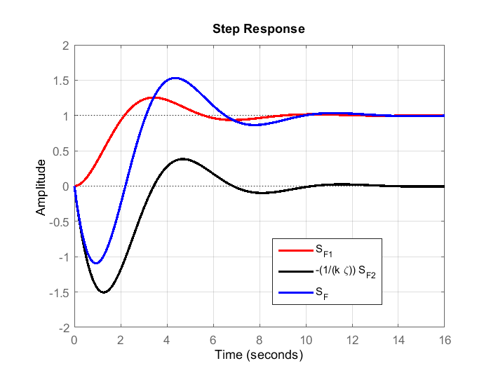
The step responses of the functions $W_{F1}$ , (scaled) $W_{F2}$ , and $W_{F}$ are shown below.

Figure 4: The step responses of the functions $W_{F1}$ , (scaled) $W_{F2}$ , and $W_{F}$ .

This graph is generated by using the MATLAB code given below.

clear,clc
zeta=0.4
omega_n=3
k=1
s=tf('s')

W1=1/(s^2+2*zeta*s+1)
W2=(1/(k*zeta))*s*W1
W3=W1+W2

figure(1)
hold on
step(W1,'r')
step(W2,'k')
step(W3,'b')

Nonminimum Phase Zeros – Effect on the Transient Response

So far, we considered zeros in the left half of the complex plane. Next, we explain the effect of zeros that are in the right half of the complex plane. The zeros in the right half of the complex plane are called nonminimum phase zeros. Systems with nonminimum phase zeros are called nonminimum phase systems and control design for such systems is more challenging compared to the systems without nonminimum phase zeros.

Consider the system given below.

(30) $\begin{align*}S_{F}=\frac{1-\frac{s}{k\zeta \omega_{n}}}{(\frac{s}{\omega_{n}})^2+2\zeta (\frac{s}{\omega_{n}})+1}\end{align*}$

where the zero is given by $s=k\zeta \omega_{n}$ . That is, the zero is in the right half of the complex plane.

By using the substitution (16), we can write the transfer function as follows

(31) $\begin{align*}S_{F}=\frac{1}{v^2+2\zeta v+1} -\frac{1}{k\zeta}\cdot \frac{v}{v^2+2\zeta v+1} \end{align*}$

By using the previously defined transfer functions

(32) $\begin{align*}W_{F1}=\frac{1}{v^2+2\zeta v+1}, \; W_{F2}= \frac{v}{v^2+2\zeta v+1}=v\cdot W_{F1}\end{align*}$

We can write (31), as follows

(33) $\begin{align*}S_{F}=W_{F1}-\frac{1}{k\zeta} W_{F2}= W_{F1}-\frac{1}{k\zeta} \cdot v \cdot W_{F1}\end{align*}$

Consequently, the analysis presented in the previous section also applies to this case. The difference is that the second transfer function in (33) has a negative sign. This means that the step response of the system will initially go in the negative direction since this negative term originating from the derivative dominates the beginning of the transient process. This is numerically illustrated in the figure below.

Figure 5: Step response of the non-minimum phase system.

The code for generating the above figure is given below.

clear,clc
zeta=0.4
omega_n=3
k=1
s=tf('s')
S1=1/(s^2+2*zeta*s+1)
S2=(1/(k*zeta))*s*S1
S=S1-S2
figure(1)
hold on
step(S1,'r')
step(-S2,'k')
step(S,'b')
grid

In Fig. 5, the blue line represents the step response of the system $S_{F}$ . From Fig. 5 we can observe that this response first goes in the negative direction. This is a direct consequence of the nonminimum phase zero. In some applications, this phenomenon can cause damage and should be properly addressed and taken into account when designing the control system.

Zero close to the real pole attenuates the effect of that pole on the system response

Zeros Tend to Increase the Overshoot of the System

Nonminimum Phase Zeros – Effect on the Transient Response

admin

You might also like

Simulation of Ordinary Differential Equations (ODEs) with Time-varying Coefficients and Time-varying Inputs in MATLAB

Introduction to Eigen C++ Matrix Library

Solve Systems of Nonlinear Equations in Python by Using FSOLVE