Bagging Method for Ensemble Machine Learning in Python and Scikit-learn

In this machine learning tutorial, we explain the basics of the bagging machine learning method for improving prediction performance. We explain how to implement the bagging method in Python and the Scikit-learn machine-learning library. The YouTube video accompanying this tutorial is given below. The GitHub page with all the codes is given here.

Basics of Sampling with Replacement, Bootstrapping, and Bagging Methods

Let us assume that we have a set of data samples. We call this data set the original data set. The bagging method consists of the following steps:

1. Create N random datasets from the original data set by using the bootstrapping method (with replacement).
2. Train a single classifier on a single data set. After this step, we have N trained classifiers that are trained on N different data sets coming from the original data set.
3. For a given test sample, predict the class label by aggregating the predictions of all N trained classifiers. In this step, to select the class label prediction we can use the voting strategy (statistical mode).

The word “bagging” is forged by combining the words bootstrap and aggregating.

First, we need to explain the step 1. That is, we need to explain the bootstrap approach for selecting random samples. This approach is based on random sampling with replacement and it creates a series of datasets with the same or a smaller number of samples than the number of samples in the original data set. These datasets are called bootstrapped datasets. Let us explain this random selection process graphically. Consider Fig. 1.

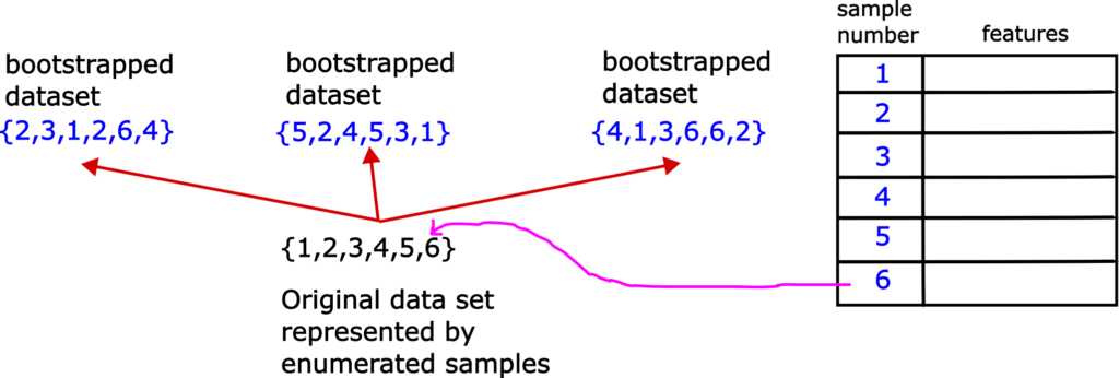
Let us assume that we have the original data set with 6 samples, enumerated from 1 to 6. Let us first form the first data set on the left. We first randomly pick a sample from the original data set. This sample is 2. Then, we return this sample to the original data set, and repeat the selection procedure again. That is, we do not exclude 2 from future selection. Next randomly selected sample is 3. After selecting this sample, we return it to the original data set. Next selected sample is 1. After selecting this sample we return it to the original data set. Next randomly selected sample is 2. Note that we have selected number 2 in the first selection step. We return number 2 to the original data set, and select in the same manner number 6 and number 4. In the same manner, we form other two bootstrapped data sets. That is the whole idea of bootstrap sampling. It is fairly simple. Note that is perfectly OK to have duplicates of samples in the bootstrapped data sets.

After we have created the bootstrapped data sets, we train classifiers on such data sets. This is illustrated in the figure below.

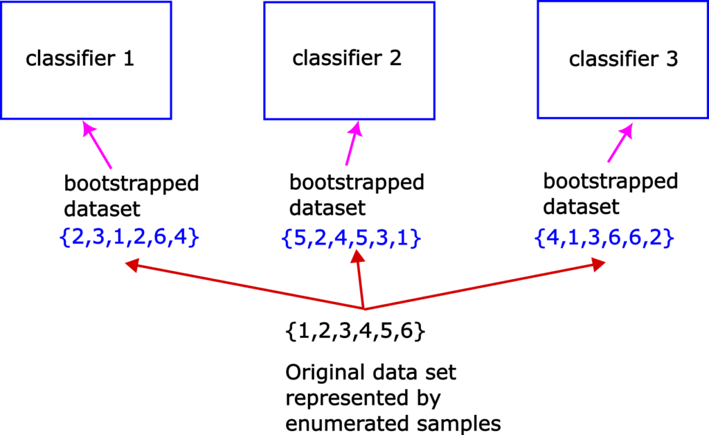
We basically train a single classifier on a single bootstrapped data set. Since they are trained on different data sets these classifiers will most likely give different predictions in the testing phase that is explained in the sequel.

Finally, let us explain the prediction step. Let us assume that the problem at hand is a binary classification problem. That is, that we only have two classes to predict: class 1 and class 2. Now, let us assume that we need to predict an appropriate class label for sample 7, that is not used during the training process. This sample can be a part of a test data set that is not used for training and it is used to evaluate the performance of the final trained models. This is shown in Fig. 3 below.

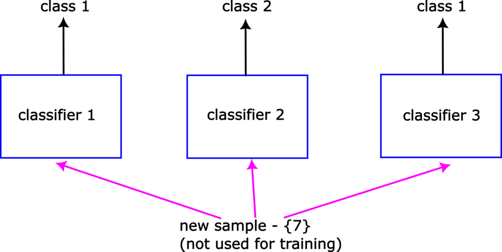
The trained classifier 1 will that the sample 7 belongs to to the class 1. The trained classifier 2 will predict that sample 7 belongs to the class 2, and the trained classifier 3 will predict that the sample 7 belongs to the class 1. The bagging classifier will take these predictions into account and it will select class 1 as the final prediction since majority of classifiers have selected this class.

We have explained the basics of bagging ensemble learning. The bagging estimator is usually used to reduce the variance of base classifiers. This is achieved by sampling the original data set, and by training the base classifiers on different data sets.

Python and Scikit-learn Implementation of Bagging Classification Method

The GitHub page with all the codes is given here. We create two bagging classifiers. The first classifier is based on decision tree base classifiers. The second classifier is based on support vector machine base classifiers. In both cases, we create 50 base classifiers. Then, we train these two classifiers on the same training data set generated from the original data set. After training these classifiers, we predict their performance by using the test data set that is completely different from the training data set. We use the accuracy measure to quantify the classifier prediction performance.

We test the performance of the constructed bagging classifiers by using the Moons data set illustrated in the figure below.

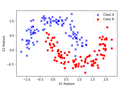
This data set is explained in our previous tutorial which can be found over here. This data set is a part of the Scikit-learn library. The importance of this data set lies in the fact that the samples of two classes are not linearly separable. That is, we cannot draw a linear line that will completely separate two classes. Consequently, basic classifiers such as linear logistic regression will not perform well on this data set. Consequently, we need to use more advanced classifiers in order to accurately distinguish samples of two classes.

Next, we present the code. First, we import the necessary libraries.

# support vector machine classifier
# https://scikit-learn.org/stable/modules/generated/sklearn.svm.SVC.html
from sklearn.svm import SVC

# decision tree classifier
# https://scikit-learn.org/stable/modules/generated/sklearn.tree.DecisionTreeClassifier.html
from sklearn.tree import DecisionTreeClassifier

# bagging classifier
# https://scikit-learn.org/stable/modules/generated/sklearn.ensemble.BaggingClassifier.html
from sklearn.ensemble import BaggingClassifier

# data set database for generating different data sets for testing the algorithms
# https://scikit-learn.org/stable/datasets.html
from sklearn import datasets
# accuracy_score metric to test the performance of the classifier
# https://scikit-learn.org/stable/modules/generated/sklearn.metrics.accuracy_score.html
from sklearn.metrics import accuracy_score
# train_test split
# https://scikit-learn.org/stable/modules/generated/sklearn.model_selection.train_test_split.html
from sklearn.model_selection import train_test_split
# standard scaler used to scale and standardize the data set
# https://scikit-learn.org/stable/modules/generated/sklearn.preprocessing.StandardScaler.html
from sklearn.preprocessing import StandardScaler 

# function for visualizing the classification areas
from functions import visualizeClassificationAreas

Not that besides importing the sklean functions, we also import “visualizeClassificationAreas” function. This function is used for visualizing the decision boundaries and classification results. Also, this function should be defined in a separate Python file that we call “functions.py”. The function is given below.

# -*- coding: utf-8 -*-
"""
This file contains the function for visualizing the classification regions

"""

def visualizeClassificationAreas(usedClassifier,XtrainSet, ytrainSet,XtestSet, ytestSet, filename='classification_results.png', plotDensity=0.01 ):
    '''
    This function visualizes the classification regions on the basis of the provided data
 
    usedClassifier      - used classifier
 
    XtrainSet,ytrainSet - train sets of features and target classes 
                        - the region colors correspond to to the class numbers in ytrainSet
 
    XtestSet,ytestSet   - test sets for visualizng the performance on test data that is not used for training
                        - this is optional argument provided if the test data is available
    
    filename            - file name with the ".png" extension to save the classification graph
 
    plotDensity         - density of the area plot, smaller values are making denser and more precise plots
 
    IMPORTANT COMMENT:  -If the number of classes is larger than the number of elements in the list 
                    caller "colorList", you need to increase the number of colors in 
                    "colorList"
                    - The same comment applies to "markerClass" list defined below
 
    '''
    import numpy as np
    import matplotlib.pyplot as plt    
    # this function is used to create a "cmap" color object that is used to distinguish different classes
    from matplotlib.colors import ListedColormap 
     
    # this list is used to distinguish different classification regions
    # every color corresponds to a certain class number
    colorList=["blue", "green", "orange", "magenta", "purple", "red"]
    # this list of markers is used to distingush between different classe
    # every symbol corresponds to a certain class number
    markerClass=['x','o','v','#','*','>']
     
    # get the number of different classes 
    classesNumbers=np.unique(ytrainSet)
    numberOfDifferentClasses=classesNumbers.size
                  
    # create a cmap object for plotting the decision areas
    cmapObject=ListedColormap(colorList, N=numberOfDifferentClasses)
                  
    # get the limit values for the total plot
    x1featureMin=min(XtrainSet[:,0].min(),XtestSet[:,0].min())-0.5
    x1featureMax=max(XtrainSet[:,0].max(),XtestSet[:,0].max())+0.5
    x2featureMin=min(XtrainSet[:,1].min(),XtestSet[:,1].min())-0.5
    x2featureMax=max(XtrainSet[:,1].max(),XtestSet[:,1].max())+0.5
         
    # create the meshgrid data for the classifier
    x1meshGrid,x2meshGrid = np.meshgrid(np.arange(x1featureMin,x1featureMax,plotDensity),np.arange(x2featureMin,x2featureMax,plotDensity))
         
    # basically, we will determine the regions by creating artificial train data 
    # and we will call the classifier to determine the classes
    XregionClassifier = np.array([x1meshGrid.ravel(),x2meshGrid.ravel()]).T
    # call the classifier predict to get the classes
    predictedClassesRegion=usedClassifier.predict(XregionClassifier)
    # the previous code lines return the vector and we need the matrix to be able to plot
    predictedClassesRegion=predictedClassesRegion.reshape(x1meshGrid.shape)
    # here we plot the decision areas
    # there are two subplots - the left plot will plot the decision areas and training samples
    # the right plot will plot the decision areas and test samples
    fig, ax = plt.subplots(1,2,figsize=(15,8))
    ax[0].contourf(x1meshGrid,x2meshGrid,predictedClassesRegion,alpha=0.3,cmap=cmapObject)
    ax[1].contourf(x1meshGrid,x2meshGrid,predictedClassesRegion,alpha=0.3,cmap=cmapObject)
     
    # scatter plot of features belonging to the data set 
    for index1 in np.arange(numberOfDifferentClasses):
        ax[0].scatter(XtrainSet[ytrainSet==classesNumbers[index1],0],XtrainSet[ytrainSet==classesNumbers[index1],1], 
                   alpha=1, c=colorList[index1], marker=markerClass[index1], 
                   label="Class {}".format(classesNumbers[index1]), edgecolor='black', s=80)
         
        ax[1].scatter(XtestSet[ytestSet==classesNumbers[index1],0],XtestSet[ytestSet==classesNumbers[index1],1], 
                   alpha=1, c=colorList[index1], marker=markerClass[index1],
                   label="Class {}".format(classesNumbers[index1]), edgecolor='black', s=80)
         
    ax[0].set_xlabel("Feature X1",fontsize=14)
    ax[0].set_ylabel("Feature X2",fontsize=14)
    ax[0].text(0.05, 0.05, "Decision areas and TRAINING samples", transform=ax[0].transAxes, fontsize=14, verticalalignment='bottom')
    ax[0].legend(fontsize=14)
     
    ax[1].set_xlabel("Feature X1",fontsize=14)
    ax[1].set_ylabel("Feature X2",fontsize=14)
    ax[1].text(0.05, 0.05, "Decision areas and TEST samples", transform=ax[1].transAxes, fontsize=14, verticalalignment='bottom')
    #ax[1].legend()
    plt.savefig(filename,dpi=500)

This function takes as inputs

1. “usedClassifier” – the classifier object
2. “XtrainSet”, “ytrainSet”, “XtestSet”, and “ytestSet” – input and output data sets
3. filename=’classification_results.png’ – this is the name of the image file that is produces by this function. The function will produce an image similar to the one shown below (this image will be explained later in the text).

We explain later in the text how to use this function.

The next steps are to load the Moons data set, split the data set into training and test data sets, and scale the features of the data sets. The following code lines perform these steps.

# load the data set
# Moons data set
# https://aleksandarhaber.com/scatter-plots-for-classification-problems-in-python-and-scikit-learn/
# https://scikit-learn.org/stable/modules/generated/sklearn.datasets.make_moons.html

# Moons data set
Xtotal, Ytotal = datasets.make_moons(n_samples=400, noise = 0.15)

# split the data set into training and test data sets
Xtrain, Xtest, Ytrain, Ytest = train_test_split(Xtotal, Ytotal, test_size=0.2)

# create a standard scaler
scaler1=StandardScaler()
# scale the training and test input data
# fit_transform performs both fit and transform at the same time
XtrainScaled=scaler1.fit_transform(Xtrain)
# here we only need to transform
XtestScaled=scaler1.transform(Xtest)

As mentioned previously, the Scikin-learn library contains an extensive database of different data sets for testing classification algorithms. We use the function “make_moons” to generate the Moons data set that is shown in Fig. 4. Then, we use the function “train_test_split” to split the data into training and test data sets. The training data set is used to train (fit) the model. The test data set is used to test the performance of the final trained model on the data set that is not used during the training process. Then, by using “StandardScaler()” we scale the input feature data. The standard scaler will remove the non-zero mean from the data set and scale the samples in the data set such that they have a unit variance. Then we fit the scaler and transform the training data set by using “fit_transform”. Also, we scale the test data set. The need for scaling of the data set is clearly explained in our previous tutorial.

Next, we define two bagging classifiers, train them, and use them for prediction.

# Define the bagging classifier by using the decision tree base classifier
# define the base classifier
# max_depth=None means that nodes are expanded until all leaves are pure
treeCLF = DecisionTreeClassifier(criterion='entropy',max_depth=None,random_state=42)
BaggingCLF_tree=BaggingClassifier(treeCLF,n_estimators=50,max_samples=0.5,bootstrap=True,n_jobs=-1)
# max samples=0.5 means that the number of random samples drawn from the original data set is equal to 
# 0.5*X.shape[0], where X is the input data set of samples (same applies to the output data set)
# n_jobs=-1 - means using all the processors to do computations
# note that since the decision tree base classifier implements predict_proba() method
# then the predicted class is selected as the class with the highest mean probability

# Define the bagging classifier by using the support vector machine base classifier
# define the base classifier
SVMCLF=SVC()
# define the bagging classifier
BaggingCLF_SVM=BaggingClassifier(SVMCLF,n_estimators=50,max_samples=0.5,bootstrap=True,n_jobs=-1)


# create a list of classifier tuples
# (classifier name, classifier object)
classifierList=[('Bagging_Tree',BaggingCLF_tree),('Bagging_SVM',BaggingCLF_SVM)]

# this dictionary is used to store the classification scores
classifierScore={}

# here we iterate through the classifiers and compute the accuracy score
# and store the accuracy store in the list
for nameCLF,CLF in classifierList:
    CLF.fit(XtrainScaled,Ytrain)
    CLF_prediction=CLF.predict(XtestScaled)
    classifierScore[nameCLF]=accuracy_score(Ytest,CLF_prediction)

To define the bagging classifier, we first need to define the base classifier. For example, the following two code lines define the base classifier and the bagging classifier:

treeCLF = DecisionTreeClassifier(criterion='entropy',max_depth=None,random_state=42)
BaggingCLF_tree=BaggingClassifier(treeCLF,n_estimators=50,max_samples=0.5,bootstrap=True,n_jobs=-1)

The base classifier is the decision tree classifier, create by using the function “DecisionTreeClassifier()”. As the criterion for forming the tree, we use “entropy”. The bagging classifier is created by using the function “BaggingClassifier()”, with the following input parameters:

• “treeCLF” is the name of the previously defined decision tree base estimator
• “n_estimators=50” – means that we will train 50 base classifiers
• “max_samples=0.5” – means that the bootstrapped data sets will have 0.5Xtrain.shape[0] samples. That is, their dimensions will be 50% smaller than the dimension of the original data set.
• “bootstrap=True” means that we are sampling the bootstrapped data sets with replacement.
• “n_jobs=-1” means that we are using all available CPUs to train the base classifiers in parallel.

In the same manner we define the support vector machine base classifier and we train the bagging classifier “BaggingCLF_SVM” by using support vector machine base classifier. Here, it should be noted that since the decision tree classifier implements the predict_proba() method, the class labels are predicted as the classes with the highest mean probability. That is, the bagging classifier based on the decision trees is not using hard voting based on binary class outputs.

The list “classifierList” contains tuples of classifier names and classifier objects. The dictionary “classifierScore” is used to store the classifier scores that are computed in the for loop. We use the accuracy measure to quantify the bagging classifier performance. The accuracy is computed by using the predicted classes and output test classes. By running the code, we obtain the following results:

{‘Bagging_Tree’: 0.9875, ‘Bagging_SVM’: 0.9875}

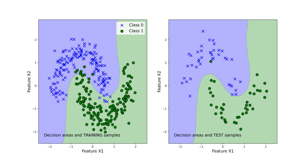
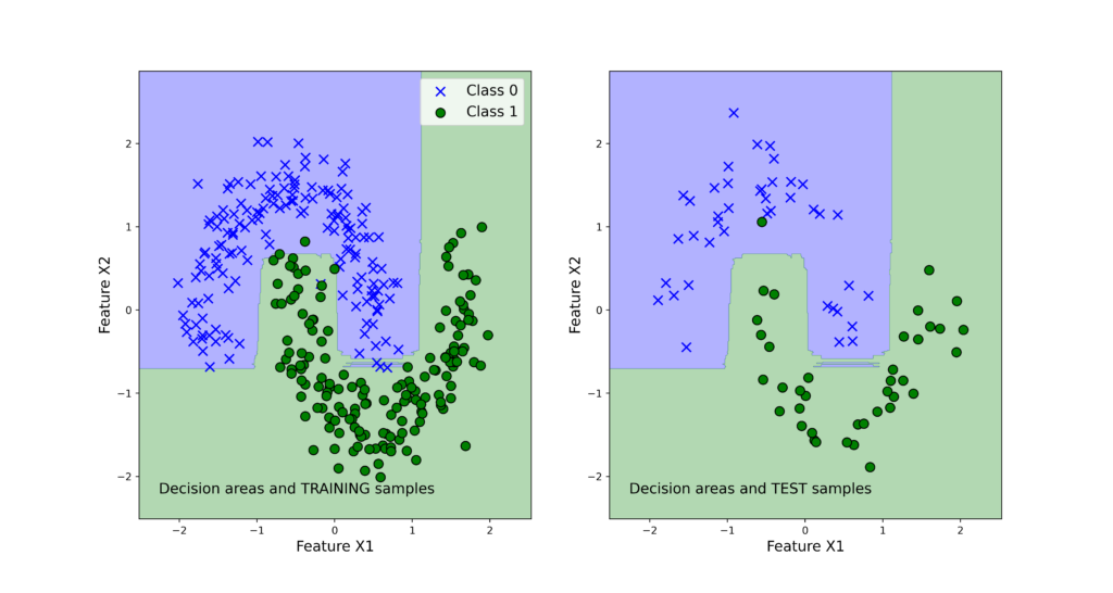
We can observe that both classifiers perform very good on the test data set. Next, we use the function “visualizeClassificationAreas” to visualize the performance of the classifiers. We can use the following two code lines too visualize the classification performance

# visualize the classification regions
visualizeClassificationAreas(BaggingCLF_tree,XtrainScaled, Ytrain,XtestScaled, Ytest, filename='classification_results_Bagging_Tree.png', plotDensity=0.01)
visualizeClassificationAreas(BaggingCLF_SVM,XtrainScaled, Ytrain,XtestScaled, Ytest, filename='classification_results_Bagging_SVM.png', plotDensity=0.01)

The figures below show the classification performance.