Ensemble Learning in Scikit-learn and Python: Voting Classifiers – Machine Learning Tutorials – Fusion of Engineering, Control, Coding, Machine Learning, and Science

In this tutorial, we explain the basics of voting classifiers and explain how to implement them in the Scikit-learn machine-learning library. The YouTube video accompanying this tutorial is given below. All the codes presented in this tutorial are given on the GitHub page.

Basics of Ensemble Learning and Voting Classifiers

Let us suppose that we ask a question to a large number of people. Most likely, a single individual will not give us the most appropriate answer. However, if we can somehow analyze all the answers and pick up either the most frequent answer, or pick up the answer according to some weighted measure, then most likely such an answer will be the correct answer. This approach is a very well-known approach in statistics, and it is often referred to as the wisdom of the crowd approach.

Loosely speaking that is the main idea of ensemble learning. We train a number of predictors on the same data set, or on smaller data sets that are samples from the same larger data set, and then we combine the predictions of all the predictors in order to choose the most appropriate prediction. There are a number of approaches for implementing this idea. In this tutorial, we focus on voting classifiers.

The idea of the voting classifiers is very simple. We train different classifiers on the same data set. Classifiers can be of completely different types, such as for example support vector machine, logistic regression, decision trees, random forests, etc., classifiers. Also, the classifiers can be of the same type, however, the parameters of the classifiers can be different. For example, we can train a series of decision trees with different parameters. After we train the classifiers, we predict the class label by using the majority vote strategy or the soft voting strategy. In this tutorial, we focus on the majority vote strategy since it is simple and easy-to understand. You can read more about soft voting strategy here.

The majority of vote strategy selects the final predicted class label of an input sample, by analyzing the class label predictions of all the predictors in the ensemble of classifiers, and by simply choosing the class label that appears most often. For example, let us say that we have 5 binary classifiers shown in the figure below.

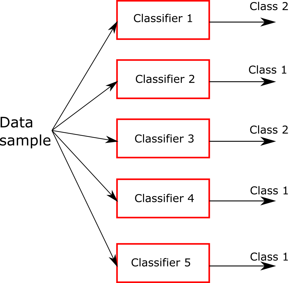
Figure 1: Illustration of the voting classifier principle

Every classifier can predict either the class 1 or the class 2. The majority vote classifier will then select the class 1 because three classifiers predict this class, and two classifiers predict the class 2. That is the basic idea of the majority vote classifier. In the sequel, we explain how to implement the voting classifier in Python. As the result, of our implementation, we will be able to generate the classification results shown below (this graph will be explained in the next section).

Figure 2: Classification results of the Moons data set.

Python and Scikit-learn Implementation of the Voting Classifier

Here, we explain how to implement the voting classifier in Python by using the Scikit-learn library. The GitHub page with all the codes is given here.

Here is the main idea

1.) We create three classifiers: support vector machine classifier, logistic regression classifier, and random forest classifier.
2.) We create a voting classifier by aggregating these three classifiers in a single classifier.
3.) We compare the predictions of all four classifiers by using the accuracy measure.
4.) We plot the decision regions.

First, we import the necessary libraries:

# support vector machine classifier
# https://scikit-learn.org/stable/modules/generated/sklearn.svm.SVC.html
from sklearn.svm import SVC
# logistic regression classifier
# https://scikit-learn.org/stable/modules/generated/sklearn.linear_model.LogisticRegression.html
from sklearn.linear_model import LogisticRegression
# random forest classifer
# https://scikit-learn.org/stable/modules/generated/sklearn.ensemble.RandomForestClassifier.html
from sklearn.ensemble import RandomForestClassifier
# voting classifier 
# https://scikit-learn.org/stable/modules/generated/sklearn.ensemble.VotingClassifier.html
from sklearn.ensemble import VotingClassifier
# data set database for generating different data sets for testing the algorithms
# https://scikit-learn.org/stable/datasets.html
from sklearn import datasets
# accuracy_score metric to test the performance of the classifier
# https://scikit-learn.org/stable/modules/generated/sklearn.metrics.accuracy_score.html
from sklearn.metrics import accuracy_score
# train_test split
# https://scikit-learn.org/stable/modules/generated/sklearn.model_selection.train_test_split.html
from sklearn.model_selection import train_test_split
# standard scaler used to scale and standardize the data set
# https://scikit-learn.org/stable/modules/generated/sklearn.preprocessing.StandardScaler.html
from sklearn.preprocessing import StandardScaler 

# function for visualizing the classification areas
from functions import visualizeClassificationAreas

Note that from the file “functions.py”, we import the function “visualizeClassificationAreas”. This function is given below and it is used to plot the decision regions.

def visualizeClassificationAreas(usedClassifier,XtrainSet, ytrainSet,XtestSet, ytestSet, filename='classification_results.png', plotDensity=0.01 ):
    '''
    This function visualizes the classification regions on the basis of the provided data
 
    usedClassifier      - used classifier
 
    XtrainSet,ytrainSet - train sets of features and target classes 
                        - the region colors correspond to to the class numbers in ytrainSet
 
    XtestSet,ytestSet   - test sets for visualizng the performance on test data that is not used for training
                        - this is optional argument provided if the test data is available
    
    filename            - file name with the ".png" extension to save the classification graph
 
    plotDensity         - density of the area plot, smaller values are making denser and more precise plots
 
    IMPORTANT COMMENT:  -If the number of classes is larger than the number of elements in the list 
                    caller "colorList", you need to increase the number of colors in 
                    "colorList"
                    - The same comment applies to "markerClass" list defined below
 
    '''
    import numpy as np
    import matplotlib.pyplot as plt    
    # this function is used to create a "cmap" color object that is used to distinguish different classes
    from matplotlib.colors import ListedColormap 
     
    # this list is used to distinguish different classification regions
    # every color corresponds to a certain class number
    colorList=["blue", "green", "orange", "magenta", "purple", "red"]
    # this list of markers is used to distingush between different classe
    # every symbol corresponds to a certain class number
    markerClass=['x','o','v','#','*','>']
     
    # get the number of different classes 
    classesNumbers=np.unique(ytrainSet)
    numberOfDifferentClasses=classesNumbers.size
                  
    # create a cmap object for plotting the decision areas
    cmapObject=ListedColormap(colorList, N=numberOfDifferentClasses)
                  
    # get the limit values for the total plot
    x1featureMin=min(XtrainSet[:,0].min(),XtestSet[:,0].min())-0.5
    x1featureMax=max(XtrainSet[:,0].max(),XtestSet[:,0].max())+0.5
    x2featureMin=min(XtrainSet[:,1].min(),XtestSet[:,1].min())-0.5
    x2featureMax=max(XtrainSet[:,1].max(),XtestSet[:,1].max())+0.5
         
    # create the meshgrid data for the classifier
    x1meshGrid,x2meshGrid = np.meshgrid(np.arange(x1featureMin,x1featureMax,plotDensity),np.arange(x2featureMin,x2featureMax,plotDensity))
         
    # basically, we will determine the regions by creating artificial train data 
    # and we will call the classifier to determine the classes
    XregionClassifier = np.array([x1meshGrid.ravel(),x2meshGrid.ravel()]).T
    # call the classifier predict to get the classes
    predictedClassesRegion=usedClassifier.predict(XregionClassifier)
    # the previous code lines return the vector and we need the matrix to be able to plot
    predictedClassesRegion=predictedClassesRegion.reshape(x1meshGrid.shape)
    # here we plot the decision areas
    # there are two subplots - the left plot will plot the decision areas and training samples
    # the right plot will plot the decision areas and test samples
    fig, ax = plt.subplots(1,2,figsize=(15,8))
    ax[0].contourf(x1meshGrid,x2meshGrid,predictedClassesRegion,alpha=0.3,cmap=cmapObject)
    ax[1].contourf(x1meshGrid,x2meshGrid,predictedClassesRegion,alpha=0.3,cmap=cmapObject)
     
    # scatter plot of features belonging to the data set 
    for index1 in np.arange(numberOfDifferentClasses):
        ax[0].scatter(XtrainSet[ytrainSet==classesNumbers[index1],0],XtrainSet[ytrainSet==classesNumbers[index1],1], 
                   alpha=1, c=colorList[index1], marker=markerClass[index1], 
                   label="Class {}".format(classesNumbers[index1]), edgecolor='black', s=80)
         
        ax[1].scatter(XtestSet[ytestSet==classesNumbers[index1],0],XtestSet[ytestSet==classesNumbers[index1],1], 
                   alpha=1, c=colorList[index1], marker=markerClass[index1],
                   label="Class {}".format(classesNumbers[index1]), edgecolor='black', s=80)
         
    ax[0].set_xlabel("Feature X1",fontsize=14)
    ax[0].set_ylabel("Feature X2",fontsize=14)
    ax[0].text(0.05, 0.05, "Decision areas and TRAINING samples", transform=ax[0].transAxes, fontsize=14, verticalalignment='bottom')
    ax[0].legend(fontsize=14)
     
    ax[1].set_xlabel("Feature X1",fontsize=14)
    ax[1].set_ylabel("Feature X2",fontsize=14)
    ax[1].text(0.05, 0.05, "Decision areas and TEST samples", transform=ax[1].transAxes, fontsize=14, verticalalignment='bottom')
    #ax[1].legend()
    plt.savefig(filename,dpi=500)

The following code lines import the data sets for classification and split the data into train and test data sets.

# Iris data set
#dataSet=datasets.load_iris()
# input data for classification
#Xtotal=dataSet['data'][:, 1:3]
#Ytotal=dataSet['target']

# Moons data set
Xtotal, Ytotal = datasets.make_moons(n_samples=200, noise = 0.15)


# split the data set into training and test data sets
Xtrain, Xtest, Ytrain, Ytest = train_test_split(Xtotal, Ytotal, test_size=0.4)

Note that we are currently using the Moons data set. We explained how to generate this data set in our previous tutorial. We have also tested the codes on the Iris data set (currently it is commented). The Moons data set is interesting since it is a binary classification problem that is not linearly separable. We used this data set in our previous tutorial and the samples of the Moons data set are shown in the figure below.

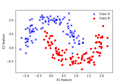
Consequently, since the classes are not linearly separable, linear classifiers such as the classical logistic regression method will not produce the best results.

Next, we scale the data. This step is explained in our previous tutorial. The code is given below.

# create a standard scaler
scaler1=StandardScaler()
# scale the training and test input data
# fit_transform performs both fit and transform at the same time
XtrainScaled=scaler1.fit_transform(Xtrain)
# here we only need to transform
XtestScaled=scaler1.transform(Xtest)

Next, we create three classifiers:

# create the classifiers
# support vector machines
SVMCLF=SVC(decision_function_shape='ovo')
# logistic regression
LogisticCLF=LogisticRegression(random_state=42)
# random forrest classifier
ForestCLF=RandomForestClassifier(n_estimators=30)

Next, we create the voting classifier on the basis of these classifiers. Then, in the for loop we train all 4 classifiers by using the training data, and make predictions on the basis of the test data.

# create a list of classifier tuples
# this list is used to form the voting classifier
# (classifier name, classifier object)
classifierTypeNameInitial=[('SVM',SVMCLF),('LogisticRegression',LogisticCLF),('RandomForest',ForestCLF)]
# here we create the voting classifier
VotingCLF=VotingClassifier(estimators=classifierTypeNameInitial, voting='hard')

# create the final list of tuples of classifiers
classifierTypeNameTotal=classifierTypeNameInitial+[('Voting',VotingCLF)]

# this dictionary is used to store the classification scores
classifierScore={}

# here we iterate through the classifiers and compute the accuracy score
# and store the accuracy store in the list
for nameCLF,CLF in classifierTypeNameTotal:
    CLF.fit(XtrainScaled,Ytrain)
    CLF_prediction=CLF.predict(XtestScaled)
    classifierScore[nameCLF]=accuracy_score(Ytest,CLF_prediction)

Note that to creating the voting classifier, we first had to create a list of tuples of 3 base classifiers. The first entry of the name is the classifier name that can be arbitrary, and the second entry is the classifier object. The code is given below.

# create a list of classifier tuples
# this list is used to form the voting classifier
# (classifier name, classifier object)
classifierTypeNameInitial=[('SVM',SVMCLF),('LogisticRegression',LogisticCLF),('RandomForest',ForestCLF)]
# here we create the voting classifier
VotingCLF=VotingClassifier(estimators=classifierTypeNameInitial, voting='hard')

If we print the “classifierScore” dictionary that stores the accuracy results, we will obtain

{‘SVM’: 0.975,
‘LogisticRegression’: 0.9,
‘RandomForest’: 0.9625,
‘Voting’: 0.9375}

Note that the voting classifier does not give the best results. This might be due to several reasons. One of the reasons is that we only have three base classifiers. Then, the logistic regression is not an appropriate classifier for the problem (remember that the problem is not linearly separable, see figure 3) and this fact biases the voting classifier results toward incorrect predictions.

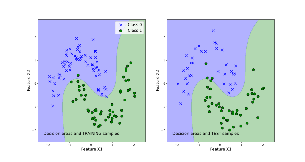
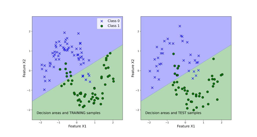
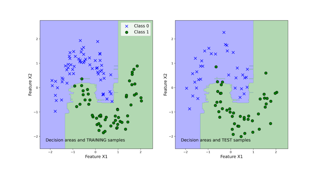
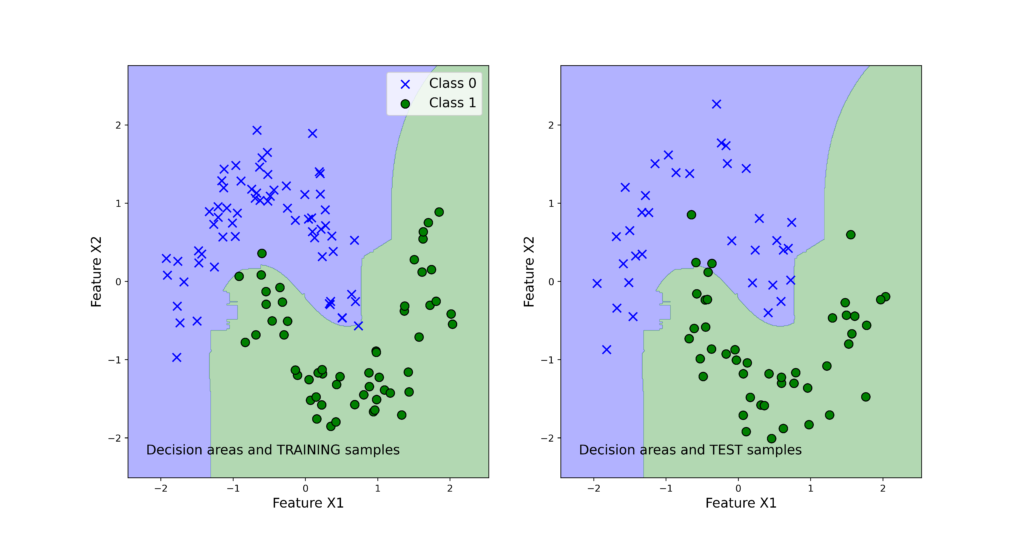
We can visualize the classification regions by using these code lines

# visualize the classification regions

visualizeClassificationAreas(SVMCLF,XtrainScaled, Ytrain,XtestScaled, Ytest, filename='classification_results_svm.png', plotDensity=0.01 )
visualizeClassificationAreas(LogisticCLF,XtrainScaled, Ytrain,XtestScaled, Ytest, filename='classification_results_logistic.png', plotDensity=0.01 )
visualizeClassificationAreas(ForestCLF,XtrainScaled, Ytrain,XtestScaled, Ytest, filename='classification_results_forest.png', plotDensity=0.01 )
visualizeClassificationAreas(VotingCLF,XtrainScaled, Ytrain,XtestScaled, Ytest, filename='classification_results_voting.png', plotDensity=0.01 )

The following 4 graphs illustrate the classification results. The left panels show the training data set. The right panels show the test data sets. We also plot the decision regions. We can observe that support vector machines produce the best results and the logistic regression produces the worst results.