Introduction to Rotation Matrices in Robotics – Fusion of Engineering, Control, Coding, Machine Learning, and Science

In this post, we explain:

How to derive rotation matrices
How to transform vectors between two rotated coordinate systems.

A YouTube video accompanying this post is given below.

Rotation matrices are important for modeling robotic systems and for solving a number of problems in robotics.

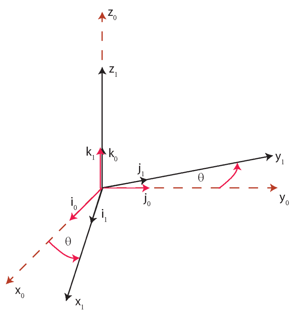
Consider Fig. 1 below.

Two coordinate systems rotated for the angle of $\theta$ around the $z_{0}$ axis.

We have two coordinate systems. The coordinate system $X_{0}Y_{0}Z_{0}$ is fixed. This coordinate system is called the inertial or reference coordinate system. Note that in robotics, coordinate systems are also called frames. The coordinate system $X_{1}Y_{1}Z_{1}$ is rotated for the angle $\theta$ with respect to the coordinate system $X_{1}Y_{1}Z_{1}$ around the $z_{0}$ axis. The vectors $i_{0}$ , $j_{0}$ , and $k_{0}$ are the unit vectors of the coordinate axes $X_{0}$ , $Y_{0}$ , and $Z_{0}$ . On the other hand, the vectors $i_{1}$ , $j_{1}$ , and $k_{1}$ are the unit vectors of the coordinate axes $X_{1}$ , $Y_{1}$ , and $Z_{1}$ .

Consider the vector $\mathbf{p}$ that rotates together with the frame $X_{1}Y_{1}Z_{1}$ and that is fixed with respect to this frame. This vector is shown in the figure below.

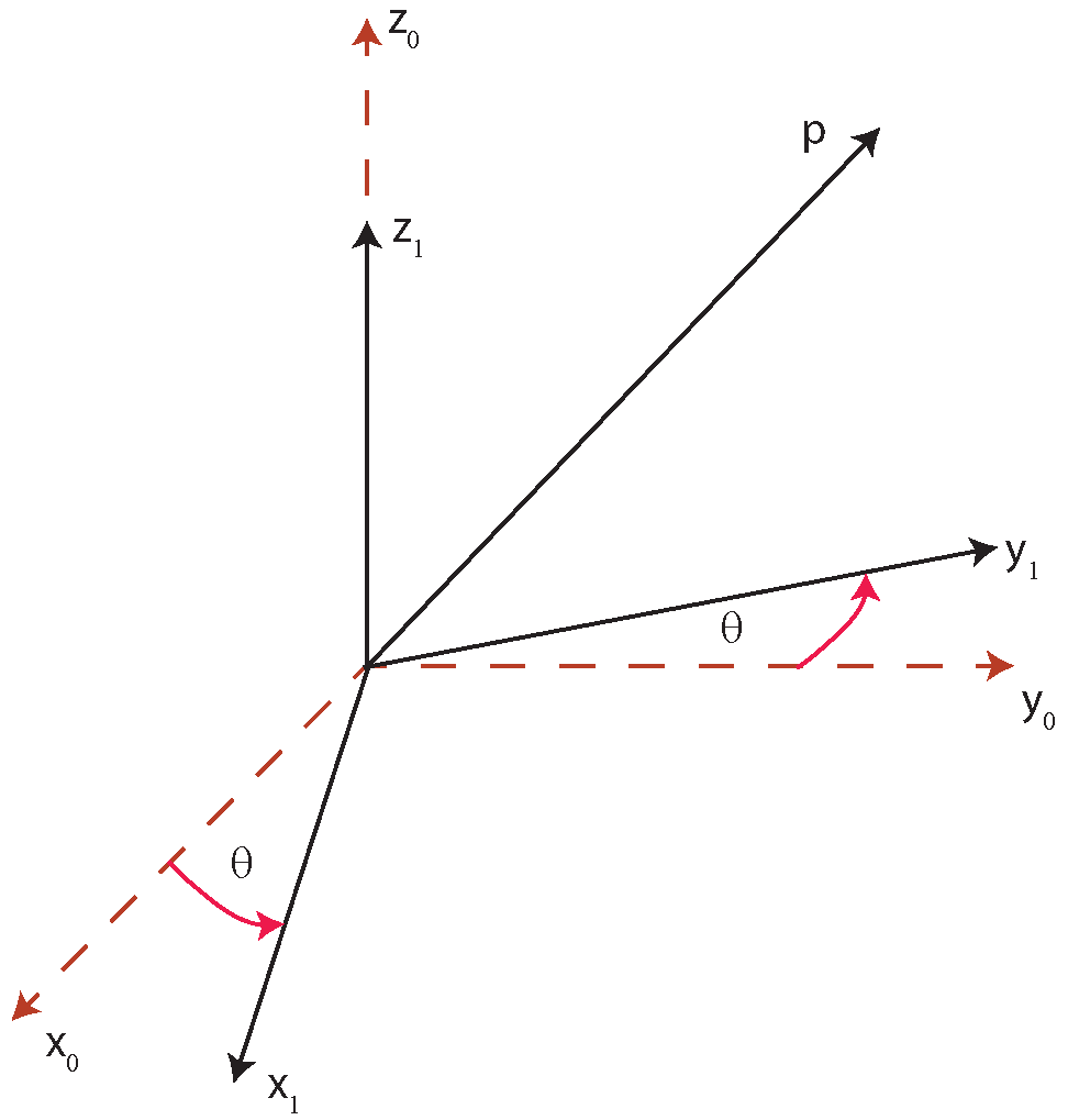
Vector $p$ rotating together with the frame $X_{1}Y_{1}Z_{1}$ .

Problem: Knowing the coordinates of the vector $p$ in the frame $X_{1}Y_{1}Z_{1}$ , and the angle of rotation $\theta$ , represent this vector in the frame $X_{0},Y_{0}, Z_{0}$ .

The representation of the vector $\mathbf{p}$ in the frame $X_{1}Y_{1}Z_{1}$ is

(1) $\begin{align*}\leftindex^{1}{\mathbf{p}}= p_{x_{1}} \mathbf{i}_{1}+ p_{y_{1}} \mathbf{j}_{1} + p_{z_{1}} \mathbf{k}_{1} \end{align*}$

where the notation $\leftindex^{1}{\mathbf{p}}$ stands for the representation of the vector $\mathbf{p}$ in the frame $1$ . And the scalars $p_{x_{1}}$ , $p_{y_{1}}$ , and $p_{z_{1}}$ are the projections. We want to compute this representation of the vector $\mathbf{p}$ in the frame $X_{0}Y_{0}Z_{0}$

(2) $\begin{align*}\leftindex^{0}{\mathbf{p}}= p_{x_{0}} \mathbf{i}_{0}+p_{y_{0}}\mathbf{j}_{0}+p_{z_{0}}\mathbf{k}_{0}\end{align*}$

From (2) and (1), we have

(3) $\begin{align*} p_{x_{0}} = \leftindex^{1}{\mathbf{p}} \cdot \mathbf{i}_{0} = p_{x_{1}} \mathbf{i}_{1} \cdot \mathbf{i}_{0} + p_{y_{1}} \mathbf{j}_{1}\cdot \mathbf{i}_{0} + p_{z_{1}} \mathbf{k}_{1}\cdot \mathbf{i}_{0} \\ p_{y_{0}} = \leftindex^{1}{\mathbf{p}} \cdot \mathbf{j}_{0} = p_{x_{1}} \mathbf{i}_{1} \cdot \mathbf{j}_{0} + p_{y_{1}} \mathbf{j}_{1}\cdot \mathbf{j}_{0} + p_{z_{1}} \mathbf{k}_{1}\cdot \mathbf{j}_{0} \\ p_{z_{0}} = \leftindex^{1}{\mathbf{p}} \cdot \mathbf{k}_{0} = p_{x_{1}} \mathbf{i}_{1} \cdot \mathbf{k}_{0} + p_{y_{1}} \mathbf{j}_{1}\cdot \mathbf{k}_{0} + p_{z_{1}} \mathbf{k}_{1}\cdot \mathbf{k}_{0} \end{align*}$

where the notation $\mathbf{i}_{1} \cdot \mathbf{i}_{0}$ is used to denote the scalar product between vectors. The last equation can be represented in the vector form

(4) $\begin{align*}\underbrace{\begin{bmatrix} p_{x_{0}} \\ p_{y_{0}} \\ p_{z_{0}} \end{bmatrix}}_{ \leftindex^{0}{\mathbf{p}} } = \underbrace{\begin{bmatrix} \mathbf{i}_{1} \cdot \mathbf{i}_{0} & \mathbf{j}_{1} \cdot \mathbf{i}_{0} & \mathbf{k}_{1} \cdot \mathbf{i}_{0} \\ \mathbf{i}_{1} \cdot \mathbf{j}_{0} & \mathbf{j}_{1} \cdot \mathbf{j}_{0} & \mathbf{k}_{1} \cdot \mathbf{j}_{0} \\ \mathbf{i}_{1} \cdot \mathbf{k}_{0} & \mathbf{j}_{1} \cdot \mathbf{k}_{0} & \mathbf{k}_{1} \cdot \mathbf{k}_{0} \end{bmatrix}}_{\leftindex^{0}_{1}R} \underbrace{\begin{bmatrix} p_{x_{1}} \\ p_{y_{1}} \\ p_{z_{1}} \end{bmatrix}}_{ \leftindex^{1}{\mathbf{p}} } \end{align*}$

where

(5) $\begin{align*} \leftindex^{0}_{1}{R} = \begin{bmatrix} \mathbf{i}_{1} \cdot \mathbf{i}_{0} & \mathbf{j}_{1} \cdot \mathbf{i}_{0} & \mathbf{k}_{1} \cdot \mathbf{i}_{0} \\ \mathbf{i}_{1} \cdot \mathbf{j}_{0} & \mathbf{j}_{1} \cdot \mathbf{j}_{0} & \mathbf{k}_{1} \cdot \mathbf{j}_{0} \\ \mathbf{i}_{1} \cdot \mathbf{k}_{0} & \mathbf{j}_{1} \cdot \mathbf{k}_{0} & \mathbf{k}_{1} \cdot \mathbf{k}_{0} \end{bmatrix} \end{align*}$

is the rotation matrix. The notation $\leftindex^{0}_{1}{R}$ denotes the transformation from the frame $1$ (subscript) to the frame $0$ (superscript). The first column of the rotation matrix is the projection of the vector $\mathbf{i}_{1}$ onto the axes of the frame $X_{0}Y_{0}Z_{0}$ . The second column of the rotation matrix is the projection of the vector $\mathbf{j}_{1}$ onto the axes of the frame $X_{0}Y_{0}Z_{0}$ . The third column of the rotation matrix is the projection of the vector $\mathbf{k}_{1}$ onto the axes of the frame $X_{0}Y_{0}Z_{0}$ .

Now, consider Fig.1 again. Since $\mathbf{i}_{1}$ and $\mathbf{i}_{0}$ are the unit vectors, we have $\mathbf{i}_{1} \cdot \mathbf{i}_{0} = | \mathbf{i}_{1} | | \mathbf{i}_{0} |cos(\theta) = 1\cdot 1 \cdot cos(\theta) =cos(\theta)$ . That is, $\mathbf{i}_{1} \cdot \mathbf{i}_{0}$ is the projection of the vector $\mathbf{i}_{1}$ onto the vector $\mathbf{i}_{0}$ , and $\theta$ is the angle between these two vectors. By using this method, we can populate the rotation matrix as follows:

(6) $\begin{align*} \leftindex^{0}_{1}{R} = \begin{bmatrix} cos(\theta) & -sin(\theta) & 0 \\ sin(\theta) & cos(\theta) & 0 \\ 0 & 0 & 1 \end{bmatrix} \end{align*}$

Rotation matrices have the following nice property:

(7) $\begin{align*} \leftindex^{0}_{1}{R} ^{-1} = \leftindex^{0}_{1}{R}^{T}\end{align*}$

That is, they are orthonormal. The inverse of $\leftindex^{0}_{1}{R}$ is actually a transformation from the frame $0$ to the frame $1$ , to see this, multiply the equation (4) by $\leftindex^{0}_{1}{R} ^{-1}$ :