Homogeneous Transformation: Rotation and Translation – Fusion of Engineering, Control, Coding, Machine Learning, and Science

In our previous post, we have explained rotation matrices. In this post, we explain how to perform rotation and translation as a single matrix operation.

A YouTube video accompanying this post is given below.

Consider the figure below.

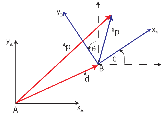
The coordinate system $B$ is translated from the coordinate system $A$ , and after that it has been rotated for the angle $\theta$ . The location of the coordinate system $B$ with respect to the coordinate system $A$ is represented by the vector $\leftindex^{A}{\mathbf{d}}$ . The notation $\leftindex^{A}{\mathbf{d}}$ means that the vector $\mathbf{d}$ is represented in the coordinate system $A$ . That is, its components (projections) are represented in the coordinate system $A$ . Similarly, the notation $\leftindex^{B}{\mathbf{p}}$ means that the vector $\mathbf{p}$ is represented in the coordinate system $A$ . Let the coordinates of the vector $\mathbf{p}$ expressed in the coordinate system $B$ be given as follows:

(1) $\begin{align*}\leftindex^{B}{\mathbf{p}} =\begin{bmatrix} p_{x_{B}} \\ p_{y_{B}} \end{bmatrix}\end{align*}$

where $p_{x_{B}}$ and $p_{y_{B}}$ are the coordinates of the vector $\mathbf{p}$ expressed in the coordinate system $B$ .

Problem 1: Given the coordinates of the vector $\leftindex^{B}{\mathbf{p}}$ , translation vector $d$ , and the angle of rotation $\theta$ , find the coordinates of the vector $\leftindex^{A}{\mathbf{p}}$ .

Solution:

(2) $\begin{align*} \leftindex^{A}{\mathbf{p}} = \leftindex^{A}{\mathbf{d}} + \leftindex^{A}_{B}{R} \cdot \leftindex^{B}{\mathbf{p}} \end{align*}$

where $\leftindex^{A}_{B}{R}$ is the rotation matrix that transforms vectors from $B$ to $A$ coordinate systems.

That is

(3) $\begin{align*}\begin{bmatrix} p_{x_{A}} \\ p_{y_{A}} \end{bmatrix} = \begin{bmatrix} d_{x_{A}} \\ d_{y_{A}} \end{bmatrix} + \begin{bmatrix} cos(\theta) & -sin(\theta) \\ sin(\theta) & cos(\theta) \end{bmatrix} \begin{bmatrix} p_{x_{B}} \\ p_{y_{B}} \end{bmatrix} \end{align*}$

If you do not remember how the rotation matrix $\leftindex^{A}_{B}{R}$

(4) $\begin{align*} \leftindex^{A}_{B}{R} = \begin{bmatrix} cos(\theta) & -sin(\theta) \\ sin(\theta) & cos(\theta) \end{bmatrix}\end{align*}$

is constructed, see our previous post.

By multiplying vectors and matrices, and by adding the results, from (3), we have

(5) $\begin{align*} p_{x_{A}} = d_{x_{A}} + cos(\theta) p_{x_{B}} - sin(\theta) p_{y_{B}} \\ p_{y_{A}} = d_{y_{A}} + sin(\theta) p_{x_{B}} + cos (\theta) p_{y_{B}} \end{align*}$

The tranformation (3), can be written as a single vector matrix multiplications. Namely, we can formally write

(6) $\begin{align*}\begin{bmatrix} \leftindex^{A}{\mathbf{p}} \\ 1 \end{bmatrix} = \begin{bmatrix} \leftindex^{A}_{B}{R} & \leftindex^{A}{\mathbf{d}} \\ \mathbf{0}_{2\times 1} & 1 \end{bmatrix} \begin{bmatrix} \leftindex^{B}{\mathbf{p}} \\ 1 \end{bmatrix} \end{align*}$

where $\mathbf{0}_{2\times 1}$ is 2 times 1 matrix of zeros. By expanding the last equation, we obtain

(7) $\begin{align*}\begin{bmatrix} p_{x_{A}} \\ p_{y_{A}} \\ 1 \end{bmatrix} = \begin{bmatrix} cos(\theta) & -sin(\theta) & d_{x_{A}} \\ sin(\theta) & cos(\theta) & d_{y_{A}} \\ 0 & 0 & 1 \end{bmatrix} \begin{bmatrix} p_{x_{B}} \\ p_{y_{B}} \\ 1 \end{bmatrix} \end{align*}$

The matrix

(8) $\begin{align*} \begin{bmatrix} cos(\theta) & -sin(\theta) & d_{x_{A}} \\ sin(\theta) & cos(\theta) & d_{y_{A}} \\ 0 & 0 & 1 \end{bmatrix} \end{align*}$

is called a homogeneous transform.

In the next post, we we will see how to use this transform to solve the forward kinematics problem of robotic manipulators.

admin

You might also like

Blender Tutorial: Correct Explanation on How to Animate Rotations of Objects

Calibration and noise reduction of distance sensors (SHARP 2Y0A21 infrared sensors)

Deformation, Strain, and Hooke’s law