Derive the Taylor Series Expansion Formula From Scratch – Must Know for Engineering Students – Fusion of Engineering, Control, Coding, Machine Learning, and Science

In this mathematics, engineering, and calculus tutorial, you will learn how the derive one of the most important formulas and approximation techniques in engineering and applied mathematics. The name of this approximation technique is the Taylor Series expansion. The YouTube tutorials accompanying this website tutorial are given below.

First, we need to provide an answer to the following question: Why do we need to learn how to derive the formula for the Taylor series expansion? Yes, that is a good question. I am well aware that some professors and teachers advise their students either to memorize the formulas or to look them up in the tables. In my opinion, both of these approaches are fundamentally wrong, and by blindly following them, you will never be able to develop a logical and precise way of thinking that is very important for being a successful engineer, scientist, or physicist. By learning how to derive formulas you will develop a logical way of thinking and you will develop an ability to mathematically analyze physical problems and mathematically formulate their solutions.

Consequently, to help you to become better engineers, scientists, and physicists, in these lectures, I will teach you how to derive important formulas that every engineer should know. Also. derivations of these formulas should be understood as mental exercises that will help you to develop important analytical skills.

Let us consider a real function $f(x)$ , where $x$ is the independent variable. Let us assume that this function is sufficiently smooth and differentiable. We can represent this function by using the Taylor series expansion given by the following equation

(1) $\begin{align*}f(x)=\sum_{i=0}^{\infty} k_{i} (x-a)^{i}\end{align*}$

where $a$ is a point about which we are approximating the function. The coefficients $k_{i}$ are determined as follows

(2) $\begin{align*}k_{i}=\frac{f^{(i)}(a)}{i !}\end{align*}$

where

(3) $\begin{align*}f^{(i)}(a)\end{align*}$

is the $i$ th derivative of the function $f(x)$ evaluated (computed) at the point $x=a$ . The Maclaurin series is obtained by using $a=0$ . That is, by approximating the function $f(x)$ around the point $x=0$ . The goal of this calculus and mathematics tutorial is to teach you how to derive the formula (2).

The Taylor series expansion is used for approximating functions. For example, we can approximate the function $f(x)$ by using a lower-order polynomial

(4) $\begin{align*}f(x)\approx k_{0}+k_{1}(x-a)+k_{2}(x-a)^{2}+k_{3}(x-a)^{3}\end{align*}$

or by using a higher-order polynomial

(5) $\begin{align*}f(x) & \approx k_{0}+k_{1}(x-a)+k_{2}(x-a)^{2}+k_{3}(x-a)^{3}+k_{4}(x-a)^{4} \\& +k_{5}(x-a)^{5}+k_{6}(x-a)^{6}+k_{7}(x-a)^{7}\end{align*}$

These approximations are illustrated in the figure below.

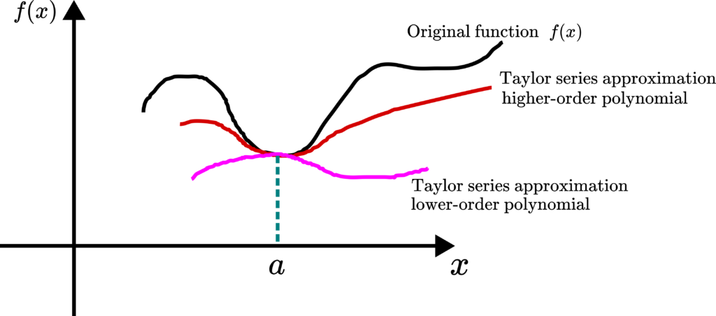
We can observe that as the order of the Taylor approximation polynomial increases, we obtain a more accurate approximation.

Let us now explain how to derive the coefficients (2). Let us expand the Taylor series formula:

(6) $\begin{align*}f(x)=k_{0}+k_{1}(x-a)+k_{2}(x-a)^{2}+k_{3}(x-a)^{3}+k_{4}(x-a)^{4}+\ldots\end{align*}$

We have

(7) $\begin{align*}f(a)=k_{0}\end{align*}$

Consequently, the coefficient $k_{0}$ is the value of the function at $a$ . This is in accordance with the formula (2). Next, let us compute the first derivative of the function (6):

(8) $\begin{align*}f'(x)=f^{(1)}(x)=k_{1}+2k_{2}(x-a)+3k_{3}(x-a)^{2}+4k_{4}(x-a)^{3}+\ldots\end{align*}$

From (8), we have

(9) $\begin{align*}f^{(1)}(a)=k_{1}\end{align*}$

Formally, from the last equation, we have

(10) $\begin{align*}k_{1}=\frac{f^{(1)}(a)}{1!}\end{align*}$

Next, by taking the derivative of (8), we obtain

(11) $\begin{align*}f^{(2)}(x)=2k_{2}+3\cdot 2 k_{3}(x-a)+4\cdot 3 k_{4}(x-a)^{2}+\ldots\end{align*}$

From the last equation, we have

(12) $\begin{align*}f^{(2)}(a)=2k_{2},\;\; k_{2}=\frac{f^{(2)}(a)}{2}\end{align*}$

By using the same principle, and by taking the derivative of (11), we obtain

(13) $\begin{align*}f^{(3)}(x)=3\cdot 2 k_{3}+4\cdot 3 \cdot 2 k_{4}(x-a)+\ldots\end{align*}$

From the last equation, we have

(14) $\begin{align*}f^{(3)}(a)=3\cdot 2 k_{3},\;\; k_{3}=\frac{f^{(3)}(a)}{3\cdot 2 \cdot 1}=\frac{f^{(3)}(a)}{3!}\end{align*}$

By using the same principle, and by taking the derivative of (13), we obtain

(15) $\begin{align*}f^{(4)}(x)=4\cdot 3 \cdot 2 k_{4}+\ldots\end{align*}$

From the last equation, we have

(16) $\begin{align*}f^{(4)}(a)=4\cdot 3 \cdot 2 k_{4},\;\; k_{4}=\frac{f^{(4)}(a)}{4\cdot 3\cdot 2 \cdot 1}=\frac{f^{(4)}(a)}{4!}\end{align*}$

By using this principle, we can show that the formula

(17) $\begin{align*}k_{i}=\frac{f^{(i)}(a)}{i !}\end{align*}$

is valid for any $i$ . This is exactly the formula (2)! In this way, we derive the general formula for the coefficients of the Taylor series expansion.

admin

You might also like

Linear Quadratic Regulator (LQR) Control of State-Space Models in Simulink and MATLAB

Thermal Deformation and Temperature-Induced Stress

Rotation Matrix Tutorial for Robotics and Aerospace Engineering – Rotation Matrix Around Y Axis