Rotation Matrix Tutorial for Robotics and Aerospace Engineering – Rotation Matrix Around Y Axis – Fusion of Engineering, Control, Coding, Machine Learning, and Science

In this robotics and aerospace lecture, we

Explain the concept of rotation matrices.
Derive the general expression for rotation matrices.
Explain that the rotation matrices are used to transform the coordinates of vectors from one to another coordinate system that are rotated with respect to each other.
Derive the expression for the rotation matrix around the y-axis.

The YouTube tutorial accompanying this tutorial is given below.

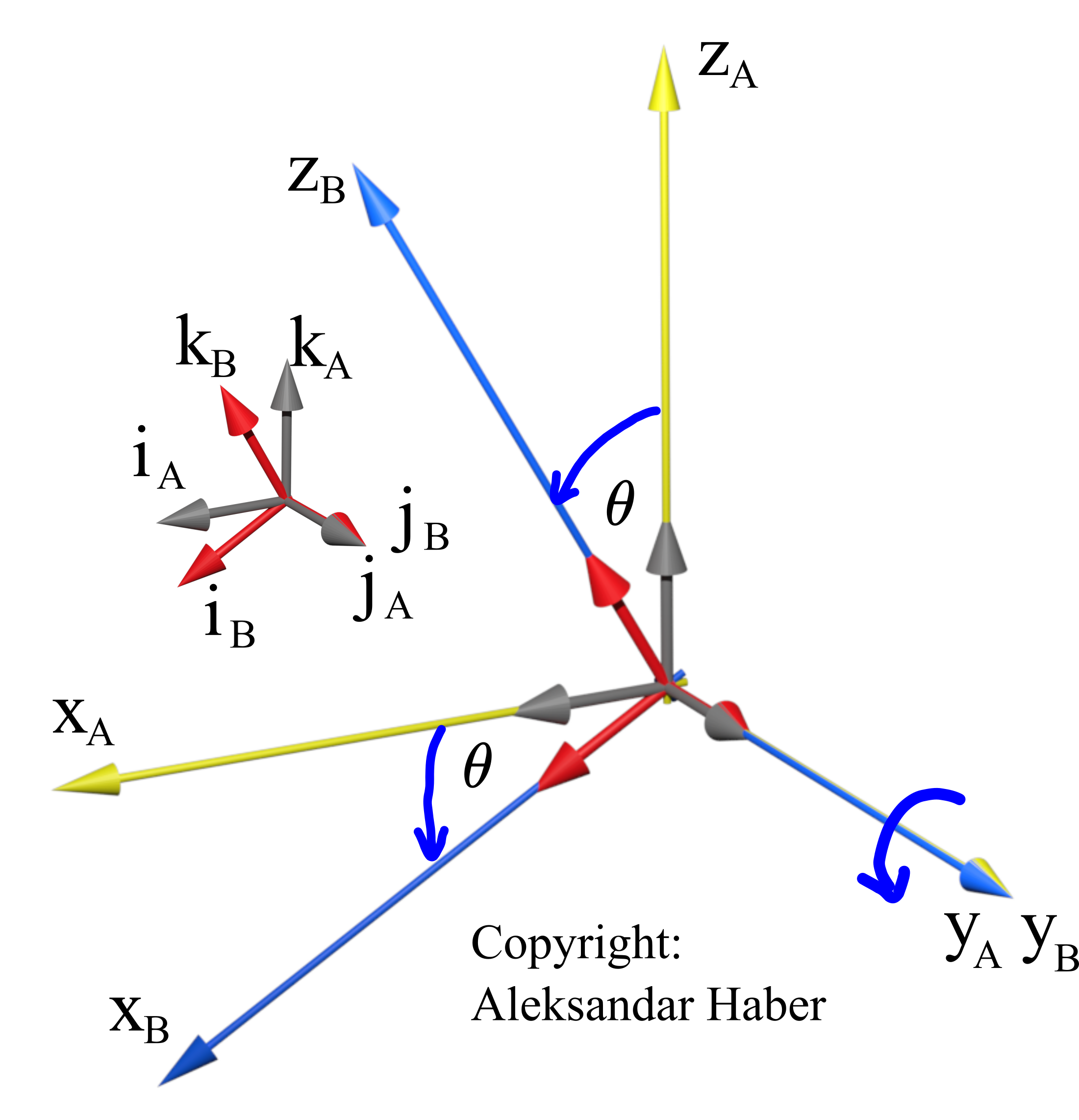
We consider the rotation of one coordinate system with respect to another one shown in the figure below.

Figure 1: Rotation of the coordinate system $B$ around the y-axis.

There are two coordinate systems A and B, with the coordinates $(x_{A},y_{A},z_{A})$ and $(x_{B},y_{B},z_{B})$ . The coordinate system $B$ is rotated with respect to the coordinate system $A$ around the axis $y_{A}$ for the angle $\theta$ . The unit vectors of the coordinate system $A$ are $\mathbf{i}_{A},\mathbf{j}_{A}$ and $\mathbf{k}_{A}$ . The unit vectors of the coordinate system $B$ are $\mathbf{i}_{B},\mathbf{j}_{B}$ and $\mathbf{k}_{B}$ . We use bold letters to denote vectors.

The figure below shows the vector $\mathbf{p}$ .

Figure 2: Rotated coordinate system with the vector $\mathbf{p}$ .

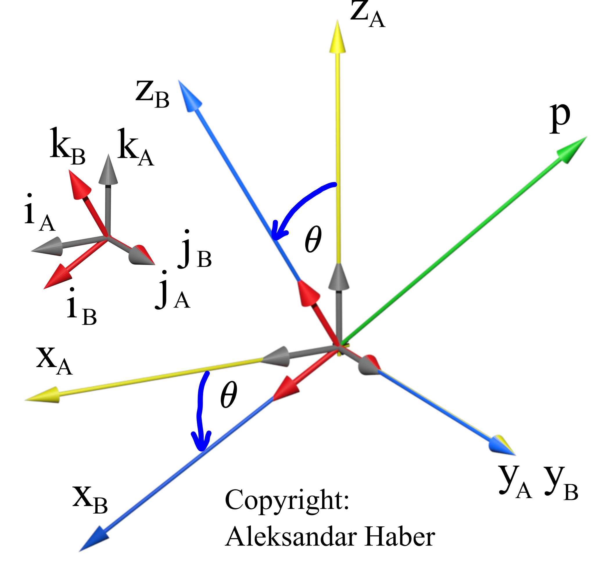Problem: Knowing the coordinates of the vector $\mathbf{p}$ in the coordinate system $B$ , and the angle of rotation $\theta$ around the axis $y_{A}$ , find the coordinates of the vector $\mathbf{p}$ in the coordinate system $A$ .

To address this problem, we introduce the following notation:

(1) $\begin{align*}\mathbf{p}^{A}=\begin{bmatrix} p_{x_{A}} \\ p_{y_{A}} \\ p_{z_{A}} \end{bmatrix}\end{align*}$

denotes the vector $\mathbf{p}$ expressed in the coordinate system $A$ . Similarly, the notation

(2) $\begin{align*}\mathbf{p}^{B}=\begin{bmatrix} p_{x_{B}} \\ p_{y_{B}} \\ p_{z_{B}} \end{bmatrix}\end{align*}$

denotes the vector $\mathbf{p}$ expressed in the coordinate system $B$ .

It should be kept in mind that the vectors $\mathbf{p}^{A}$ and $\mathbf{p}^{B}$ are actually denoting the same vector $\mathbf{p}$ only expressed in different coordinate systems. The vector $\mathbf{p}$ expressed in the coordinate system $A$ is

(3) $\begin{align*}\mathbf{p}^{A} =p_{x_{A}} \mathbf{i}_{A}+p_{y_{A}} \mathbf{j}_{A}+p_{z_{A}}\mathbf{k}_{A}\end{align*}$

The vector $\mathbf{p}$ expressed in the coordinate system $B$ is

(4) $\begin{align*}\mathbf{p}^{B} =p_{x_{B}} \mathbf{i}_{B}+p_{y_{B}} \mathbf{j}_{B}+p_{z_{B}}\mathbf{k}_{B}\end{align*}$

Here one thing should always be kept in mind. The unit vectors of both coordinate systems $A$ and $B$ are actually expressed in the same basis. That is, they are expressed by using coordinates of some other coordinate system. That is why we can mathematically write:

(5) $\begin{align*}\mathbf{p}=\mathbf{p}^{A}=\mathbf{p}^{B}\end{align*}$

That is, we have

(6) $\begin{align*}\mathbf{p}^{A}=\mathbf{p}^{B}\end{align*}$

By substituting (3) and (4) in (6), we have

(7) $\begin{align*}p_{x_{A}} \mathbf{i}_{A}+p_{y_{A}} \mathbf{j}_{A}+p_{z_{A}}\mathbf{k}_{A}=p_{x_{B}} \mathbf{i}_{B}+p_{y_{B}} \mathbf{j}_{B}+p_{z_{B}}\mathbf{k}_{B}\end{align*}$

By scalarly multiplying the equation (7) with $\mathbf{i}_{A}$ , we obtain

(8) $\begin{align*}p_{x_{A}} =p_{x_{B}} \mathbf{i}_{B}\cdot \mathbf{i}_{A}+p_{y_{B}} \mathbf{j}_{B}\cdot \mathbf{i}_{A}+p_{z_{B}}\mathbf{k}_{B}\cdot \mathbf{i}_{A}\end{align*}$

By scalarly multiplying the equation (7) with $\mathbf{j}_{A}$ , we obtain

(9) $\begin{align*}p_{y_{A}} =p_{x_{B}} \mathbf{i}_{B}\cdot \mathbf{j}_{A}+p_{y_{B}} \mathbf{j}_{B}\cdot \mathbf{j}_{A}+p_{z_{B}}\mathbf{k}_{B}\cdot \mathbf{j}_{A}\end{align*}$

By scalarly multiplying the equation (7) with $\mathbf{k}_{A}$ , we obtain

(10) $\begin{align*}p_{z_{A}} =p_{x_{B}} \mathbf{i}_{B}\cdot \mathbf{k}_{A}+p_{y_{B}} \mathbf{j}_{B}\cdot \mathbf{k}_{A}+p_{z_{B}}\mathbf{k}_{B}\cdot \mathbf{k}_{A}\end{align*}$

Let us write the equations (8), (9), and (10) together

(11) $\begin{align*}p_{x_{A}} =p_{x_{B}} \mathbf{i}_{B}\cdot \mathbf{i}_{A}+p_{y_{B}} \mathbf{j}_{B}\cdot \mathbf{i}_{A}+p_{z_{B}}\mathbf{k}_{B}\cdot \mathbf{i}_{A} \\p_{y_{A}} =p_{x_{B}} \mathbf{i}_{B}\cdot \mathbf{j}_{A}+p_{y_{B}} \mathbf{j}_{B}\cdot \mathbf{j}_{A}+p_{z_{B}}\mathbf{k}_{B}\cdot \mathbf{j}_{A} \\p_{z_{A}} =p_{x_{B}} \mathbf{i}_{B}\cdot \mathbf{k}_{A}+p_{y_{B}} \mathbf{j}_{B}\cdot \mathbf{k}_{A}+p_{z_{B}}\mathbf{k}_{B}\cdot \mathbf{k}_{A}\end{align*}$

The last three equations can be written in the matrix form as follows

(12) $\begin{align*}\begin{bmatrix}p_{x_{A}} \\p_{y_{A}} \\p_{z_{A}} \end{bmatrix} =\begin{bmatrix} \mathbf{i}_{B}\cdot \mathbf{i}_{A} & \mathbf{j}_{B}\cdot \mathbf{i}_{A} & \mathbf{k}_{B}\cdot \mathbf{i}_{A} \\ \mathbf{i}_{B}\cdot \mathbf{j}_{A} & \mathbf{j}_{B}\cdot \mathbf{j}_{A} & \mathbf{k}_{B}\cdot \mathbf{j}_{A} \\ \mathbf{i}_{B}\cdot \mathbf{k}_{A} & \mathbf{j}_{B}\cdot \mathbf{k}_{A} & \mathbf{k}_{B}\cdot \mathbf{k}_{A}\end{bmatrix}\begin{bmatrix} p_{x_{B}} \\ p_{y_{B}} \\ p_{z_{B}} \end{bmatrix}\end{align*}$

The last equation can be written compactly

(13) $\begin{align*}\mathbf{p}^{A}=R_{B}^{A}\cdot \mathbf{p}^{B}\end{align*}$

where

(14) $\begin{align*}\mathbf{p}^{A}=\begin{bmatrix}p_{x_{A}} \\p_{y_{A}} \\p_{z_{A}} \end{bmatrix},\;\; \mathbf{p}^{B}=\begin{bmatrix} p_{x_{B}} \\ p_{y_{B}} \\ p_{z_{B}} \end{bmatrix},\;\; R_{B}^{A} =\begin{bmatrix} \mathbf{i}_{B}\cdot \mathbf{i}_{A} & \mathbf{j}_{B}\cdot \mathbf{i}_{A} & \mathbf{k}_{B}\cdot \mathbf{i}_{A} \\ \mathbf{i}_{B}\cdot \mathbf{j}_{A} & \mathbf{j}_{B}\cdot \mathbf{j}_{A} & \mathbf{k}_{B}\cdot \mathbf{j}_{A} \\ \mathbf{i}_{B}\cdot \mathbf{k}_{A} & \mathbf{j}_{B}\cdot \mathbf{k}_{A} & \mathbf{k}_{B}\cdot \mathbf{k}_{A}\end{bmatrix}\end{align*}$

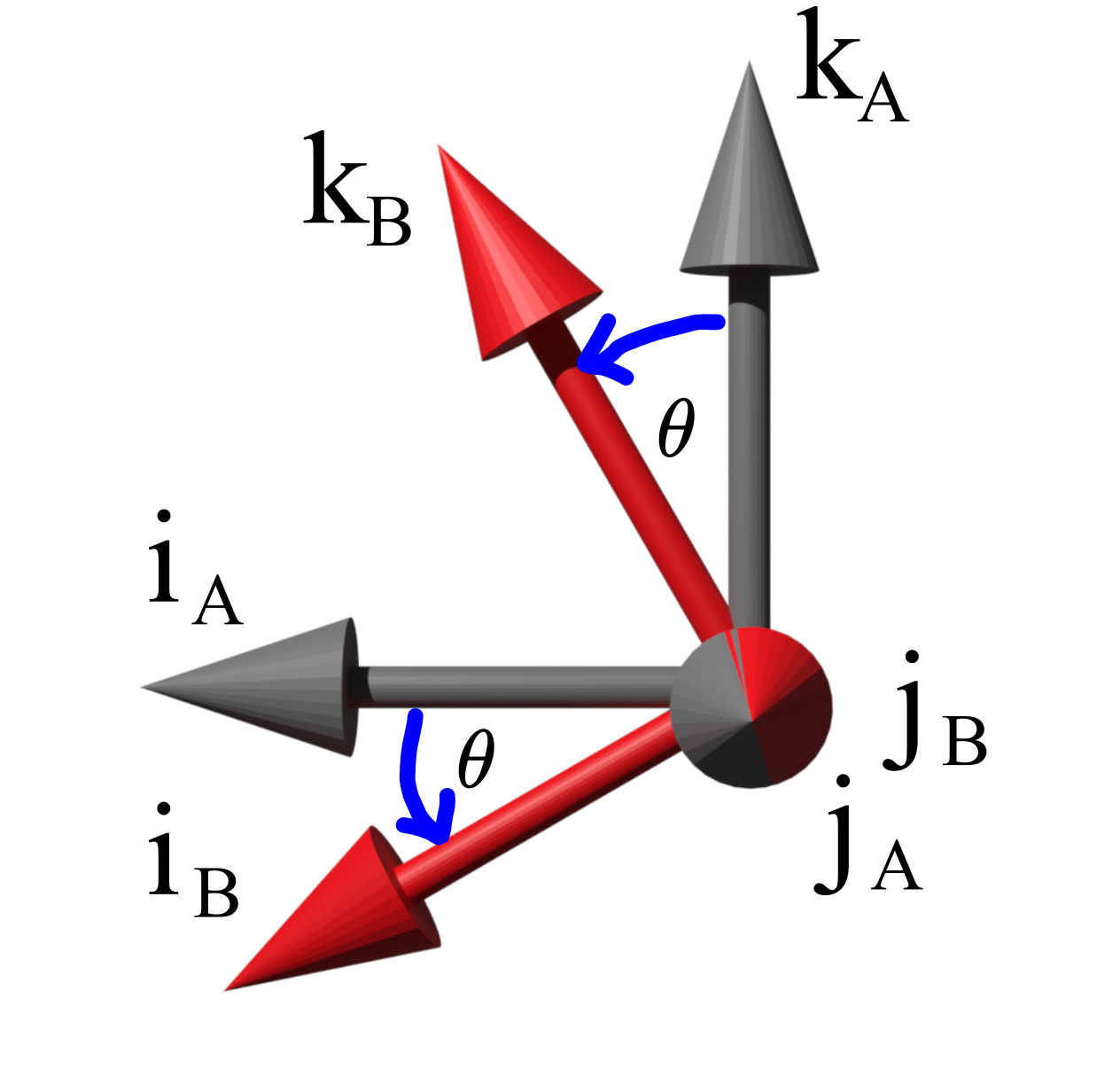
The matrix $R_{B}^{A}$ is the rotation matrix. The superscript and subscript notations in $R_{B}^{A}$ mean that the rotation matrix transforms projections of a vector from the coordinate system $B$ into the coordinate system $A$ . Let us observe the figure shown below. This figure shows the side view (from the top of the unit vector of the $y_{A}$ axis) of the unit vectors of the coordinate systems $A$ and $B$ .

Since the vectors $\mathbf{i}_{A},\mathbf{j}_{A},\mathbf{k}_{A}$ and $\mathbf{i}_{B},\mathbf{j}_{B},\mathbf{k}_{B}$ are unit vectors, we have

(15) $\begin{align*}& \mathbf{i}_{B}\cdot \mathbf{i}_{A}= \cos(\theta) ,\;\; \mathbf{j}_{B}\cdot \mathbf{i}_{A}= 0 ,\;\; \mathbf{k}_{B}\cdot \mathbf{i}_{A} =\sin(\theta) \\& \mathbf{i}_{B}\cdot \mathbf{j}_{A}= 0 ,\;\; \mathbf{j}_{B}\cdot \mathbf{j}_{A}= 1 ,\;\; \mathbf{k}_{B}\cdot \mathbf{j}_{A} = 0 \\& \mathbf{i}_{B}\cdot \mathbf{k}_{A}= -\sin(\theta) ,\;\; \mathbf{j}_{B}\cdot \mathbf{k}_{A} =0 ,\;\; \mathbf{k}_{B}\cdot \mathbf{k}_{A} = \cos(\theta)\end{align*}$

By substituting (15) in (14), we have

(16) $\begin{align*} R_{B}^{A} =\begin{bmatrix} \cos(\theta) & 0 & \sin(\theta) \\ 0 & 1 & 0 \\ -\sin(\theta) & 0 & \cos(\theta) \end{bmatrix}\end{align*}$

The matrix defined in (16) is the rotation matrix defining the rotation of two coordinate systems around the $y_{A}$ axis.

To summarize, the expression

(17) $\begin{align*}\mathbf{p}^{A}=R_{B}^{A}\cdot \mathbf{p}^{B}\end{align*}$

implements a mapping. It transforms the projections of the vector $p$ expressed in the coordinate system $B$ , into the projections of the vector $p$ expressed in the coordinate system $A$ .

Another important property of the rotation matrices is that they are orthogonal, that is,

(18) $\begin{align*}\big(R_{B}^{A}\big)^{-1}=\big( R_{B}^{A} \big)^{T}=R_{A}^{B}\end{align*}$

This is important since from (17), we can write

(19) $\begin{align*}\mathbf{p}^{A}=R_{B}^{A}\cdot \mathbf{p}^{B} \\\big( R_{B}^{A}\big)^{-1}\mathbf{p}^{A}=\mathbf{p}^{B} \\\big( R_{B}^{A}\big)^{T}\mathbf{p}^{A}=\mathbf{p}^{B} \\\mathbf{p}^{B}= R_{A}^{B}\mathbf{p}^{A} ,\;\; R_{A}^{B} =\big( R_{B}^{A}\big)^{T}\end{align*}$

More about the properties of the rotation matrices can be found here.

admin

You might also like

Extended Kalman Filter Tutorial With Example and Disciplined Python Codes – PART I -Derivation

PID Controller Discretization and Implementation in Arduino

Introduction to Rotation Matrices in Robotics