Linear Quadratic Regulator (LQR) Control of State-Space Models in Simulink and MATLAB – Fusion of Engineering, Control, Coding, Machine Learning, and Science

In this control engineering and control theory tutorial, we explain how to model and simulate Linear Quadratic Regulator (LQR) optimal controller in Simulink and MATLAB. We augment the basic LQR controller with an integral control action to improve the tracking performance of the LQR regulator. The YouTube tutorial is given below. In our next tutorial, whose link is given here, we explain how to design a pole placement controller in Simulink.

As a test case, we consider the mass-spring-damper system shown below.

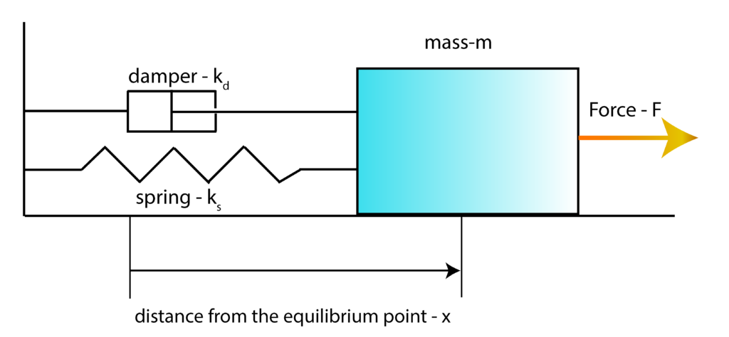
In the figure above, $x$ is the position of the point mass from its equilibrium point, $k_{d}$ is the damper constant, $k_{s}$ is the spring constant, $m$ is the mass, and $F$ is the external force applied to the point mass. The derivation of the state-space model of this system is thoroughly explained in our previous video tutorial, which can be found here. Here, for brevity and completeness of this tutorial, we briefly summarize the state-space model. By using the following state-space variables:

(1) $\begin{align*}x_{1}=x \\x_{2}=\dot{x}\end{align*}$

and the equation of motion, we obtain the following state-space model

(2) $\begin{align*}\dot{\mathbf{x}}& =A\mathbf{x}+B\mathbf{u} \\\mathbf{y}&=C\mathbf{x} \end{align*}$

where

(3) $\begin{align*}\mathbf{x}=\begin{bmatrix}x_{1} \\ x_{2} \end{bmatrix},\;\; A=\begin{bmatrix}0 & 1 \\ -\frac{k_{s}}{m} & -\frac{k_{d}}{m} \end{bmatrix},\;\; B=\begin{bmatrix} 0 \\ \frac{1}{m} \end{bmatrix},\;\; C=\begin{bmatrix}1 & 0 \end{bmatrix}\end{align*}$

Let $\mathbf{r}$ denote the reference signal. This is the signal that is set by the user and the goal is to design a feedback control algorithm that will track this signal. For that purpose, we introduce the control error (also known as the tracking error):

(4) $\begin{align*}\mathbf{e}=\mathbf{r}-\mathbf{y}\end{align*}$

Next, we introduce the integral of the control error

(5) $\begin{align*}\mathbf{x}_{i}=\int \mathbf{e} \cdot \text{d}t=\int \big( \mathbf{r}-\mathbf{y} \big) \text{d}t\end{align*}$

By taking the first derivative of the last equation, and by substituting the output equation of the state-space model in the resulting equation, we obtain

(6) $\begin{align*}\dot{\mathbf{x}}_{i}=\mathbf{r}-C\mathbf{x}\end{align*}$

By combining this equation with the state equation, we obtain the augmented system:

(7) $\begin{align*}\dot{\mathbf{x}}& =A\mathbf{x}+B\mathbf{u} \\\dot{\mathbf{x}}_{i}& =\mathbf{r} - C\mathbf{x}\end{align*}$

The last two equations can be written in the compact form

(8) $\begin{align*}\begin{bmatrix} \dot{\mathbf{x}} \\ \dot{\mathbf{x}}_{i} \end{bmatrix}=\begin{bmatrix}A & 0 \\ -C & 0 \end{bmatrix}\begin{bmatrix} \mathbf{x} \\ \mathbf{x}_{i} \end{bmatrix}+\begin{bmatrix}B \\ 0 \end{bmatrix}\mathbf{u}+\begin{bmatrix}0 \\ I \end{bmatrix}\mathbf{r}\end{align*}$

The last equation can be written compactly as follows

(9) $\begin{align*}\dot{\mathbf{x}}_{a}=A_{a}\mathbf{x}_{a}+B_{a}\mathbf{u}+B_{r}\mathbf{r}\end{align*}$

where

(10) $\begin{align*}\mathbf{x}_{a}=\begin{bmatrix} \mathbf{x} \\ \mathbf{x}_{i} \end{bmatrix},\;\; A_{a}=\begin{bmatrix}A & 0 \\ -C & 0 \end{bmatrix},\;\; B_{a}=\begin{bmatrix}B \\ 0 \end{bmatrix},\;\; B_{r}=\begin{bmatrix}0 \\ I \end{bmatrix}\end{align*}$

Here, $\mathbf{x}_{a}$ is the state of the augmented system. Here, for simplicity, while calculating the LQR controller, we will not explicitly take into account the constant reference signal $\mathbf{r}$ . This signal is implicitly taken into account by the variable $\mathbf{x}_{i}$ . The LQR controller aims at minimizing the following cost function

(11) $\begin{align*}J=\int_{0}^{\infty} \Big(\mathbf{x}_{a}^{T}Q\mathbf{x}_{a}+\mathbf{u}^{T}R\mathbf{u}+2\mathbf{x}_{a}^{T}N\mathbf{u}\Big)\text{d}t\end{align*}$

with respect to the control input $\mathbf{u}$ . The matrices $Q$ , $R$ , and $N$ are the weighting matrices selected by the user. In this tutorial, we set $N=0$ . The solution is given by the feedback control algorithm

(12) $\begin{align*}\mathbf{u}=-K\mathbf{x}_{a}\end{align*}$

where $K$ is the feedback control matrix. As we will explain later, this matrix can easily be computed by using the MATLAB function “lqr()”.

By partitioning $K$ as follows

(13) $\begin{align*}K=\begin{bmatrix}K_{x} & K_{i} \end{bmatrix}\end{align*}$

and by using the definition of $\mathbf{x}_{a}$ given in (10), we obtain

(14) $\begin{align*}\mathbf{u}=-K\mathbf{x}_{a}=-\begin{bmatrix} K_{x} & K_{i} \end{bmatrix}\begin{bmatrix} \mathbf{x} \\ \mathbf{x}_{i} \end{bmatrix}=-K_{x}\mathbf{x}-K_{i} \mathbf{x}_{i} \end{align*}$

By using (5), the last equation can be written as follows

(15) $\begin{align*}\mathbf{u}=-K_{x}\mathbf{x}-K_{i} \mathbf{x}_{i} =-K_{x}\mathbf{x}-K_{i}\int \big(\mathbf{r} - \mathbf{y} \big) \text{d}t \end{align*}$

We can clearly observe that the controller explicitly takes into account the integral of the control error. To develop a Simulink model and simulate it, we need to create a block diagram of the system and the controller. The block diagram is given below.

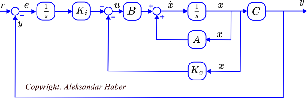
This block diagram is important for developing the Simulink model. The MATLAB script that is used to design the LQR controller is given below.

ks=1
kd=0.1
m=10

A=[0 1; -ks/m -kd/m];
B=[0; 1/m];
C=[1 0]
D=[0]

% compute the open loop poles
openLoopPoles=eig(A)

% form the augmented system
Aa=[A [0; 0]; -C 0]
Ba=[B;0]
Ca=[C, 0]
ssModel=ss(Aa,Ba,Ca,[])

% design the optimal controller
Q=[3 0 0;
    0 3 0;
    0 0 3;]
R=1;
N=zeros(3,1)
[K,~,~] = lqr(ssModel,Q,R,N)

% check the closed loop poles
eig(Aa-Ba*K)
% extract feedback matrices

Kx=K(:,1:2)
Ki=K(3)

This code, as well as the Simulink model, are explained in the YouTube tutorial given at the top of this tutorial.

admin

You might also like

Basics of Unit Conversion

Intuitive Understanding of Lyapunov’s Stability Analysis – 1D Example

Installation and Getting Started with OpenAI Gym and Frozen Lake Environment – Reinforcement Learning Tutorial