Intuitive Understanding of Lyapunov’s Stability Analysis – 1D Example – Fusion of Engineering, Control, Coding, Machine Learning, and Science

In this control engineering tutorial, we provide an intuitive understanding of Lyapunov’s stability analysis. The YouTube video accompanying this tutorial is given below.

1D Dynamical System and Analytical Solution

Let us consider the following dynamical system

(1) $\begin{align*}\dot{x}=-x\end{align*}$

Let us solve this differential equation. We have

(2) $\begin{align*}\frac{dx}{dt}=-x \\\frac{dx}{x}=-dt \\\int \frac{dx}{x} =- \int dt \\\ln (x) =-t +C \\x=e^{-t+C}\end{align*}$

where $C$ is a constant that we need to determine. We determine this constant from the initial condition. Let us assume that

(3) $\begin{align*}x(0) = x_{0}\end{align*}$

where $x_{0}\in \mathbb{R}$ is an arbitrary initial condition. It can be positive or negative. By substituting this initial condition into the last equation of (2), we obtain

(4) $\begin{align*}x(0)=x_{0}=e^{0+C}=e^{C}\end{align*}$

Consequently, the solution can be written as follows

(5) $\begin{align*}x=e^{-t}x_{0}\end{align*}$

Let us next illustrate this solution for different values of $x_{0}$ . The state trajectories are shown in the figure below.

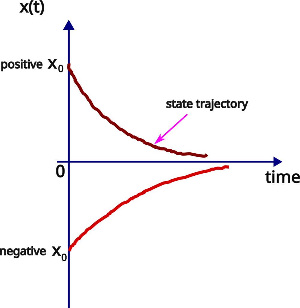
If the initial condition is positive, then the state trajectories starting from that initial condition will exponentially decrease according to the law (5). However, they will never reach zero in the final time. On the other hand, if the initial condition is negative, then the state trajectory will increase. However, it will never reach zero. That is, the state will always stay negative.

These trajectories are also illustrated in the figure below.

From this analysis, we conclude that the equilibrium point $x^{*}=0$ is asymptotically stable.

Stability Analysis Without Solving the Equation – First Approach

Let us try to analyze the stability of the equilibrium point without actually solving the differential equation (1). Here, for clarity, we write the differential equation once more

(6) $\begin{align*}\dot{x}=-x\end{align*}$

Let us assume that at a certain point in time, the state is positive. This means that $x>0$ . This implies that the right-hand side of the differential equation (6) is negative. This further implies that the derivative of the state with respect of time is negative. That is, the state decreases and approaches zero.

On the other hand, let us assume that at a certain point in time, the state is negative. This means that $x<0$ . This further implies that the first derivative is positive. This means that the state increases, and approaches zero. This is illustrated in the figure below.

By using this simple analysis, we conclude that the equilibrium point is asymptotically stable.

Stability Analysis by Using Lyapunov’s Stability Theorem

Let us recall the Lyapunov stability theorem. We introduced this theorem in our previous tutorial, which can be found here. For completeness, in the sequel, we restate the Lyapunov stability theorem.

Lyapunov (local) Stability Theorem: Consider a dynamical system

(7) $\begin{align*}\dot{\mathbf{x}}=\mathbf{f}(\mathbf{x})\end{align*}$

where $\mathbf{x}\in \mathbb{R}^{n}$ is a state vector, and $\mathbf{f}$ is a (nonlinear) vector function. Let $\mathbf{x}^{*}=0$ be an equilibrium point of (7). Let us assume that we are able to find a continuously differentiable scalar function of the state vector argument $V(\mathbf{x})$ , defined on a neighborhood set $D$ of $\mathbf{x}^{*}$ , that satisfies the following two conditions:

The function $V(\mathbf{x})$ is (locally) positive definite in $D$ . That is, $V(0)=0$ and $V(\mathbf{x})>0$ in $D-\{0\}$ for all $\mathbf{x}$ in $D$ .
The time derivative of $V(\mathbf{x})$ along state trajectories of the system is (locally) negative semi-definite in $D$ . That is, $\dot{V}(\mathbf{x})\le 0$ for all $\mathbf{x}$ in $D$ .

Then, $\mathbf{x}^{*}=0$ is stable.

In addition, if the first time derivative of $V(\mathbf{x})$ is (locally) negative definite in $D-\{0\}$ along any state trajectory of the system. That is, $\dot{V}(\mathbf{x}) < 0$ in $D-\{0\}$ , then $\mathbf{x}^{*}=0$ is asymptotically stable.

Let us select the following Lyapunov’s function candidate for our one-dimensional system:

(8) $\begin{align*}V(x)=x^2\end{align*}$

This function is positive definite everywhere, and $V(0)=0$ . The first condition is satisfied. Let us compute the time derivative of this function along the trajectories of the system. We have

(9) $\begin{align*}\dot{V}(x)=2x\dot{x}\end{align*}$

Here, while computing the first derivative of $V(x)$ , we used the chain rule. That is, we assumed that $x=x(t)$ , and consequently $V(x)=V(x(t))$ . That is, $V$ function is a composite function since $x$ depends on time. Since we are computing the first derivative along the trajectories of the system, we need to substitute the system dynamics in the last equation. By substituting (1) in the last equation, we obtain

(10) $\begin{align*}\dot{V}(x)=2x\dot{x}=2x(-x)=-2x^{2}\end{align*}$

This function is obviously negative definite everywhere. Consequently, we conclude that the function $V(x)$ is the Lyapunov function and that the system is asymptotically stable. However, can we give a physical interpretation and intuitive explanation of this stability result? The answer is yes. For that purpose, consider the figure shown below.

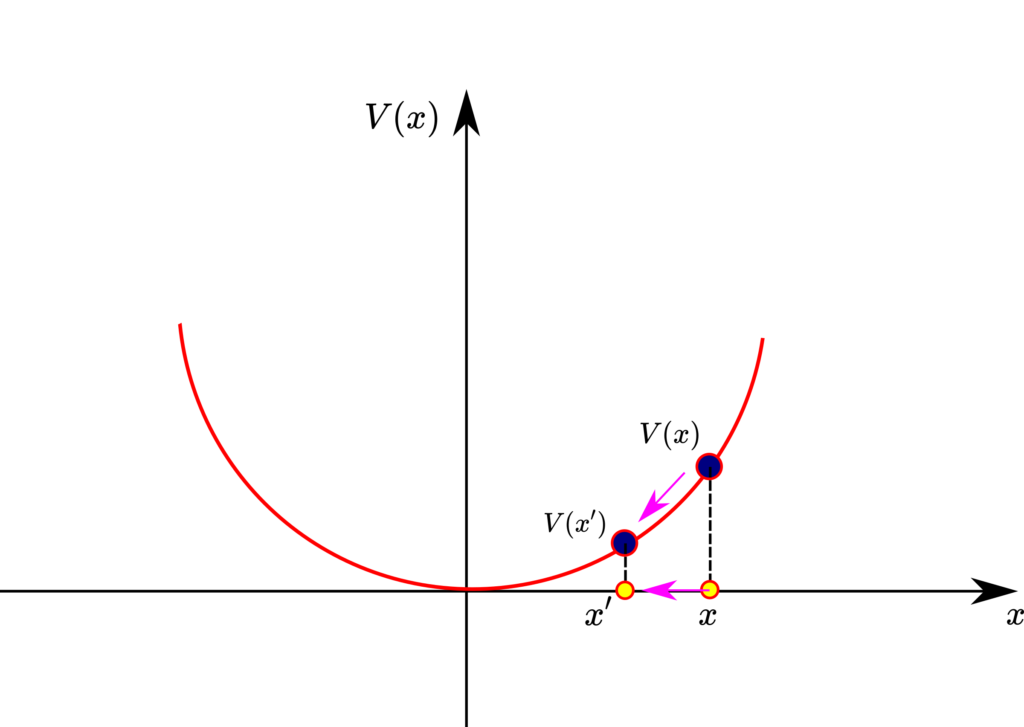
Let us assume that at the time instant $t$ , the system was at state $x$ . Then, since the system is asymptotically stable, at some other time instant $t'>t$ , the system will be in state $x'$ that is closer to the origin. In fact, the system is exponentially stable (this can be seen from the solution (5)). Consider the figure shown above. The state trajectory of the system along the x-axis can be seen as the projection of the trajectory of the ball that rolls up or down the Lyapunov function. If the time derivative of $V(x)$ is negative, this means that the ball has to role down. This in turn means that the state trajectory of the system has to approach zero equilibrium point. That is, $x$ should decrease over time. This is a very rough explanation of why the negative definiteness of the first derivative of the Lyapunov function ensures that the system trajectories are asymptotically stable. On the other hand, let us assume that the system is asymptotically stable, this means that $V(x')< V(x)$ . By using this fact, we obtain: