Magnitude (Amplitude) and Phase Response of Discrete-Time Systems and Filters – Fusion of Engineering, Control, Coding, Machine Learning, and Science

In this digital signal processing and discrete-time control tutorial, we explain how to calculate the magnitude (amplitude) and phase responses of discrete-time systems and filters. First, we briefly summarize the concept of the frequency response, and then we solve an example. We also explain the concepts of digital frequency, baseband, sampling frequency, and the relation of the digital frequency with the Nyquist frequencies and continuous time angular frequencies. In the second part of this tutorial, given here, we explain how to compute the phase and magnitude response of digital filters in Python.

The YouTube video accompanying this tutorial is given below.

Frequency Response Summary

The basic idea is to start from the transfer function of the discrete-time system that has the following form

(1) $\begin{align*}H(z)=\frac{\sum_{k=0}^{m} a_{k}z^{-k} }{\sum_{k=0}^{n}b_{k}z^{-k}}\end{align*}$

where $a_{k}$ and $b_{k}$ are real numbers or coefficients of the system (filter), and $z$ is the complex variable that is associated with the $Z$ -transform. The frequency response is obtained by substituting $z$ with

(2) $\begin{align*}z=e^{j\omega}\end{align*}$

where $j$ is the imaginary unit and $\omega$ , is often referred to as the digital frequency. Here, it should be noted that $\omega$ is in the interval $\omega \in [-\pi, +\pi ]$ . That is, we only consider this interval when computing the frequency response. The reasons for this will be explained later on in this tutorial. As a result, we obtain the following expression

(3) $\begin{align*}H(z)\Bigg|_{z=e^{j\omega}}=H(e^{j\omega})=\frac{\sum_{k=0}^{m} a_{k}e^{-j\omega k} }{\sum_{k=0}^{n}a_{k}b^{-j\omega k}}\end{align*}$

As it will become completely clear after we solve an example, the expression (3) is a complex number or better to say a complex function of $\omega$ . Consequently, we can represent the complex number (3) in the polar form

(4) $\begin{align*}H(e^{j\omega})=M(\omega)e^{j\theta (\omega)}\end{align*}$

where

$M(\omega)=|H(e^{j\omega})|$ is a function of $\omega$ that is called the magnitude response of the amplitude response of the system.
$\theta (\omega)$ is a function of $\omega$ that is called the phase response of the system.

There are a number of approaches for computing the phase and magnitude responses. We can use the polar form of a complex number to transform expressions in the numerator and denominator of $H(e^{j\omega})$ , and from there we can find the polar form of the complete expression. Another approach for computing the phase and magnitude responses is to represent the complex number $H(e^{j\omega})$ in the rectangular form

(5) $\begin{align*}H(e^{j\omega})=\Re \{H(e^{j\omega}) \}+\Im \{H(e^{j\omega}) \}\end{align*}$

where $\Re \{H(e^{j\omega}) \}$ and $\Im \{H(e^{j\omega}) \}$ are the real and imaginary parts of $H(e^{j\omega})$ . The magnitude response is then

(6) $\begin{align*}M(\omega)=\sqrt{\big( \Re \{H(e^{j\omega}) \}\big)^{2}+\big( \Im \{H(e^{j\omega}) \}\big) ^{2}}\end{align*}$

and the phase response is then computed by solving this equation

(7) $\begin{align*}\tan \left( \theta (\omega ) \right) = \frac{\Im \{H(e^{j\omega}) \}}{\Re \{H(e^{j\omega}) \}}\end{align*}$

Before we explain how to compute the frequency response it is important to clarify several important things related to the digital frequency $\omega$ . The digital frequency is defined by

(8) $\begin{align*}\omega = \omega_{c}\cdot T_{s}\end{align*}$

where $\omega_{c}$ is the continuous-time (angular or radial) frequency and $T_{s}$ is the sampling period of the discrete-time signal.

First of all, the continuous-time sinusoidal signals are quantified by the continuous-time angular frequency $\omega_{c}$ :

(9) $\begin{align*}y(t)=\sin(\omega_{c}t)\end{align*}$

where $t$ is continuous time and $\omega_{c}$ is equal to

(10) $\begin{align*}\omega_{c}=\frac{2\pi}{T_{c}}\end{align*}$

where $T_{c}$ is the period of the continuous-time sinusoidal signal. However, the period of the continuous time signal $T_{c}$ should not be confused with the sampling period $T_{s}$ . If the signal is sampled with the sampling period of $T_{s}$ , then the time is $t=nT_{s}$ , where $n$ is an integer denoting a discrete-time instant. In that case, the continuous-time signal (9) is represented by

(11) $\begin{align*}y[n]=y(nT_{s})=\sin(\omega_{c}nT_{s})=\sin(n\omega_{c}T_{s})=\sin(n\omega)\end{align*}$

where $\omega$ is the digital frequency that we introduced previously. When analyzing the frequency response of discrete-time systems or the spectrum of discrete-time signals, the digital frequency is in the following range

(12) $\begin{align*}\omega\in [-\pi, +\pi]\end{align*}$

This is due to several important reasons. First of all, when analyzing discrete-time signals, we only take into account their continuous-time pairs that are in the frequency range from zero to the continuous-time frequency $\omega_{s}/2$ , where

(13) $\begin{align*}\omega_{s}=\frac{2\pi}{T_{s}}=2\pi\cdot f_{s}\end{align*}$

is the angular sampling frequency and $f_{s}=1/T_{s}$ is the sampling frequency. The frequency $\omega_{s}/2$ or equivalently $f_{s}/2$ are called Nyquist frequencies. If we substitute $\omega_{c}$ for $\omega_{s}/2$ in (8), we obtain

(14) $\begin{align*}\omega=\frac{\omega_{s}}{2}T_{s}=\frac{2\pi}{2T_{s}}\cdot T_{s}=\pi\end{align*}$

That is, the maximal digital frequency that we can take into account is $\pi$ . On the other hand, for systems that have a real-valued impulse response, the magnitude (amplitude) response is an even function of the digital frequency, and the phase response is an odd function of the digital frequency. This means that for such systems, we can only consider the digital frequency in the range $[0,+\pi]$ when computing the frequency response. However, it is a standard practice to consider the full frequency range:

(15) $\begin{align*}-\pi \le \omega \le +\pi\end{align*}$

The interval (15) is often referred to as the digital baseband or simply as baseband.

Another important thing to keep in mind is that due to sampling, the frequency response of the system is periodic with the period of $2\pi$ in the digital frequency domain, or with the equivalent period of $\omega_{s}$ in the continuous frequency domain. That is, the magnitude and phase responses in the baseband, repeat themselves with the period of $2\pi$ . Due to all these reasons, we only compute the frequency response for the frequencies in the baseband (15).

Also, the discrete-time transfer function $H(z)$ is the Z-transform of the impulse response of the discrete-time system. Consequently, the function $H(e^{j\omega})$ is the frequency spectrum of the impulse response sequence of the system.

Example of Computing Phase and Frequency Response of Discrete-time (Digital) System (Filter)

Let us consider the following discrete-time system

(16) $\begin{align*}y[n]=\frac{1}{2}\big(x[n]-x[n-1] \big)\end{align*}$

where $x[n]$ is the input sequence and $y[n]$ is the output sequence. The first step is to derive the transfer function. To do that we apply the Z-transform to (16)

(17) $\begin{align*}\mathcal{Z}\{ y[n] \}=\frac{1}{2}\mathcal{Z}\{ x[n] \}-\frac{1}{2}\mathcal{Z}\{ x[n-1] \}\end{align*}$

using the following notation

(18) $\begin{align*}\mathcal{Z}\{ y[n] \}= Y(z) \\\mathcal{Z}\{ x[n] \}=X(z)\end{align*}$

, and the fact that $\mathcal{Z}\{ x[n-1] \}=z^{-1}X(z)$ , from (17), we have

(19) $\begin{align*}Y(z)=\frac{1}{2}X(z)-\frac{1}{2}z^{-1}X(z)\end{align*}$

(20) $\begin{align*}Y(z)=\frac{z-1}{2z} X(z) \end{align*}$

From the last equation, we have

(21) $\begin{align*}\frac{Y(z)}{X(z)}=H(z)=\frac{z-1}{2z}\end{align*}$

This is the transfer function of the system. Let us compute the frequency response

(22) $\begin{align*}H(e^{j\omega})=\frac{e^{j\omega}-1}{2e^{j\omega}}\end{align*}$

From the last equation, we have

(23) $\begin{align*}H(e^{j\omega})=\frac{e^{\frac{j\omega}{2}}}{2e^{j\omega}}\cdot \Big(e^{\frac{j\omega}{2}}-e^{-\frac{j\omega}{2}} \Big)\end{align*}$

The idea for this transformation is to use this formula

(24) $\begin{align*}\sin (\alpha)=\frac{e^{j\alpha}-e^{-j\alpha}}{2j}\end{align*}$

to eliminate the difference between the complex exponentials and to compute the magnitude response.

From (23), we have

(25) $\begin{align*}H(e^{j\omega}) & =\frac{e^{\frac{j\omega}{2}}}{e^{j\omega}}\cdot j \cdot \frac{\Big(e^{\frac{j\omega}{2}}-e^{-\frac{j\omega}{2}} \Big)}{2j} \\H(e^{j\omega}) & =e^{j(\frac{\omega}{2}-\omega )}\cdot e^{j\frac{\pi}{2}}\cdot\frac{\Big(e^{\frac{j\omega}{2}}-e^{-\frac{j\omega}{2}} \Big)}{2j}\end{align*}$

By using (24), from (25) we obtain

(26) $\begin{align*}H(e^{j\omega}) & =e^{j(-\frac{\omega}{2}+\frac{\pi}{2} )}\cdot \sin(\frac{\omega}{2})\end{align*}$

From this equation, we can conclude that the magnitude response is

(27) $\begin{align*}M(\theta)=|\sin(\frac{\omega}{2})|\end{align*}$

At first sight, from (26) it looks like the phase response is $\frac{\omega}{2}+\frac{\pi}{2}$ . However, this is not a correct conclusion! This is mainly because the sign of the term $\sin(\frac{\omega}{2})$ changes when $\omega$ is varied from $-\pi$ to $+\pi$ . This means that when $\sin(\frac{\omega}{2})\ge 0$

(28) $\begin{align*}H(e^{j\omega}) & = |\sin(\frac{\omega}{2})| e^{j(-\frac{\omega}{2}+\frac{\pi}{2} )} \end{align*}$

on the other hand, when $\sin(\frac{\omega}{2})< 0$

(29) $\begin{align*}H(e^{j\omega}) & = -|\sin(\frac{\omega}{2})| e^{j(-\frac{\omega}{2}+\frac{\pi}{2} )} =|\sin(\frac{\omega}{2})| e^{j(-\frac{\omega}{2}+\frac{\pi}{2} )} e^{\pm j \pi}=|\sin(\frac{\omega}{2})| e^{j(-\frac{\omega}{2}+\frac{\pi}{2} \pm \pi )} \end{align*}$

This means that the correct phase is given by

(30) $\begin{align*}\theta (\omega )& =-\frac{\omega}{2}+\frac{\pi}{2} ,\;\; \text{for} \;\; \sin(\frac{\omega}{2})>0,\;\; 0 \le \frac{\omega}{2} \le \pi \\\theta (\omega )& =-\frac{\omega}{2}+\frac{\pi}{2}\pm \pi ,\;\; \text{for} \;\; \sin(\frac{\omega}{2})<0,\;\; -\pi \le \frac{\omega}{2} \le 0\end{align*}$

(31) $\begin{align*}\theta (\omega )&=-\frac{\omega}{2}+\frac{\pi}{2} ,\;\; \text{for} \;\; 0 \le \omega \le 2\pi \\\theta (\omega )&=-\frac{\omega}{2}-\frac{\pi}{2} ,\;\; \text{for} \;\; -2\pi \le \omega \le 0\end{align*}$

or finally

(32) $\begin{align*}\theta (\omega )&=-\frac{\omega}{2}+\frac{\pi}{2} ,\;\; \text{for} \;\; 0 \le \omega \le \pi \\\theta (\omega )& =-\frac{\omega}{2}-\frac{\pi}{2} ,\;\; \text{for} \;\; -\pi \le \omega \le 0\end{align*}$

The phase and magnitude responses are shown in the figure below.

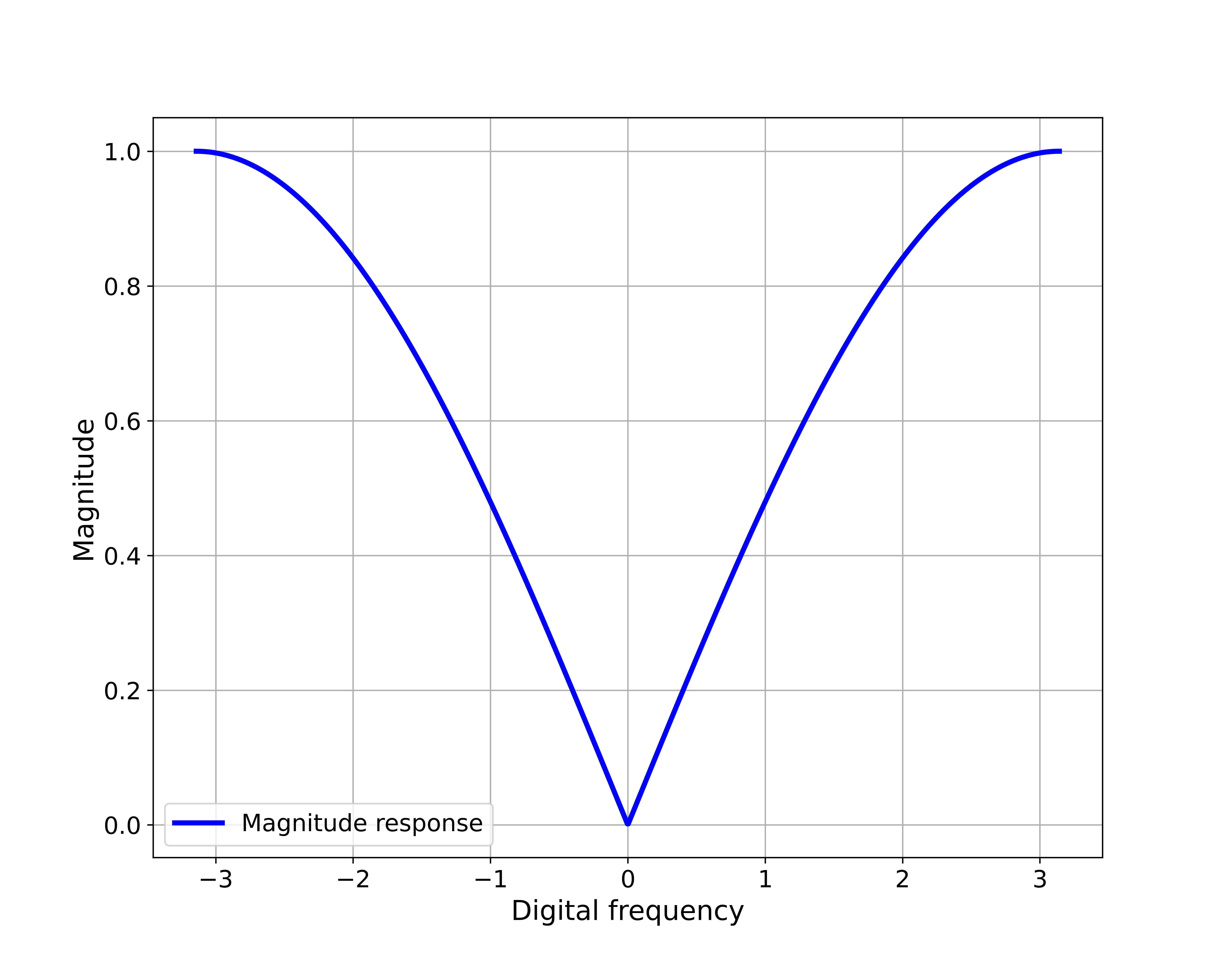
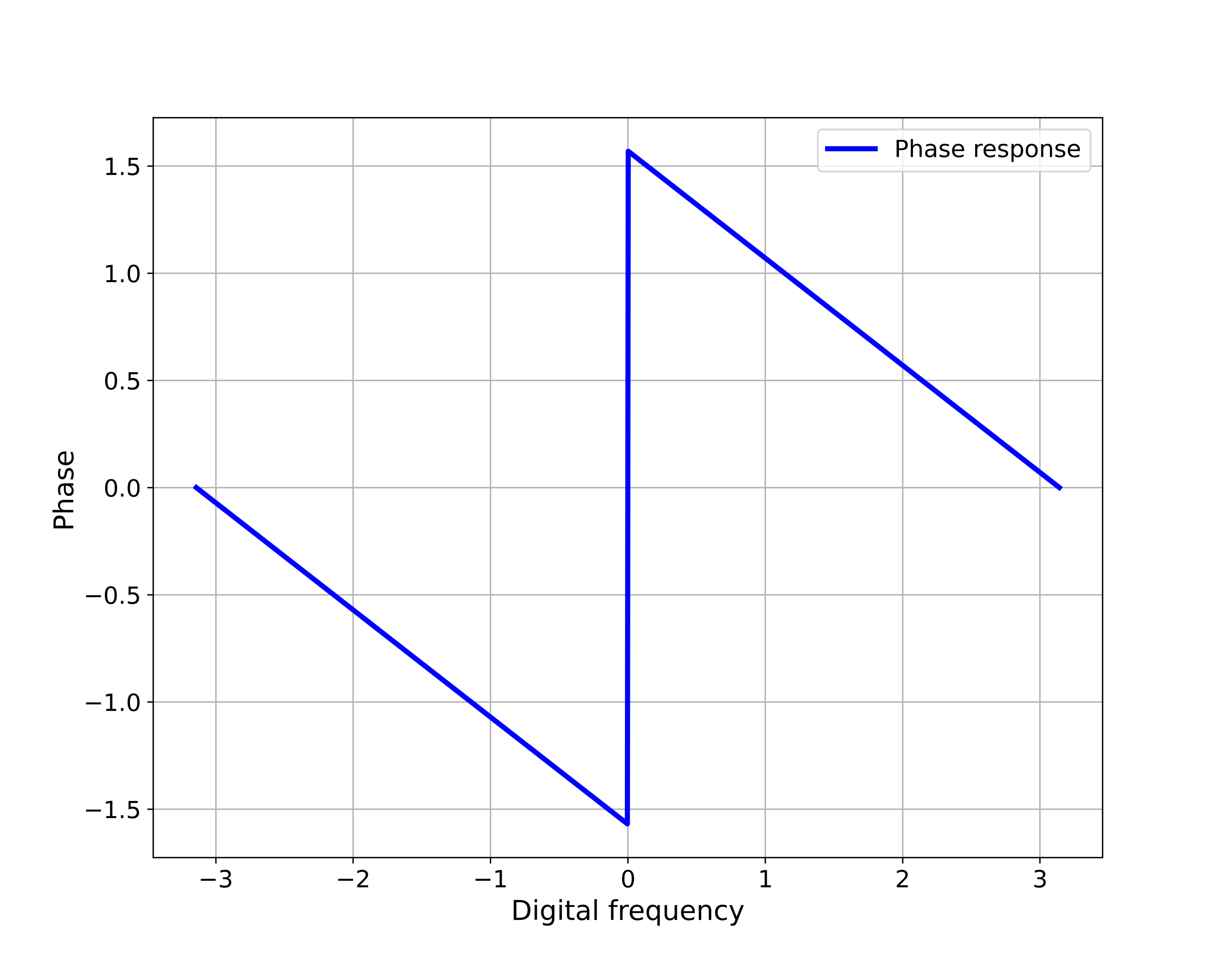
Figure 1: Magnitude response of the system (21).

Figure 2: Phase response of the system (21).

From the magnitude response, we can see that this system attenuates the low frequencies and the high frequencies are not attenuated. That is, this filter acts as a high-pass filter. These two graphs are generated by using the Python code that is explained in the tutorial given here.

Frequency Response Summary

Example of Computing Phase and Frequency Response of Discrete-time (Digital) System (Filter)

admin

You might also like

Control Systems Lecture: DC motor state-space modeling and MATLAB’s Control System Toolbox simulations

Compute Magnitude and Phase Responses (Frequency Response) of Digital Filters and Discrete-Time Systems in Python

Clear and Concise Particle Filter Tutorial with Python Implementation- Part 3: Python Implementation of Particle Filter Algorithm