Clear and Concise Particle Filter Tutorial with Python Implementation- Part 3: Python Implementation of Particle Filter Algorithm – Fusion of Engineering, Control, Coding, Machine Learning, and Science

This is the third part of the tutorial series on particle filters. In this third tutorial part, we explain how to implement the particle filter algorithm in Python. Below is the summary of all tutorial parts, their brief description, and links to their webpages. The GitHub page with the developed Python scripts that implement and test the particle filter algorithm is given here.

PART 1: In Part 1, we presented the problem formulation for estimating the state of a dynamical system by using the particle filter.

PART 2: In Part 2, we derived the particle filter algorithm. More precisely, we derived the bootstrap particle filter algorithm which is also known as the Sequential Importance Resampling (SIR) filter.

PART 3: You are currently reading Part 3. In this tutorial part, we explain how to implement the SIR particle filter algorithm in Python from scratch.

The YouTube video accompanying this webpage is given below.

Below is the video tutorial illustrating the behavior of the particle filter.

Brief Summary of Particle Filter Algorithm

Here, for completeness, we provide a brief summary of the particle filter algorithm.

Not to blur the main ideas of particle filters with too many mathematical details, in this tutorial series, we derived the particle filter algorithm for linear state-space models. However, everything explained in this tutorial series can be generalized to nonlinear systems. The particle filter is derived for the following state-space model:

(1) $\begin{align*}\mathbf{x}_{k}& =A\mathbf{x}_{k-1}+B\mathbf{u}_{k-1}+\mathbf{w}_{k-1} \\\mathbf{y}_{k}& =C\mathbf{x}_{k}+\mathbf{v}_{k}\end{align*}$

where $\mathbf{x}_{k}\in \mathbb{R}^{n}$ is the state vector at the discrete time step $k$ , $\mathbf{u}_{k-1}\in \mathbb{R}^{m_{1}}$ is the control input vector at the time step $k-1$ , $\mathbf{w}_{k-1}\in \mathbb{R}^{m_{2}}$ is the process disturbance vector (process noise vector) at the time step $k-1$ , $\mathbf{y}_{k}\in \mathbb{R}^{r}$ is the observed output vector at the time step $k$ , $\mathbf{v}_{k}\in \mathbb{R}^{r}$ is the measurement noise vector at the discrete time step $k$ , and $A$ , $B$ , and $C$ are system matrices.

It is assumed that the process disturbance vector $\mathbf{w}_{k}$ is normally distributed with zero mean and prescribed covariance matrix, that is

(2) $\begin{align*}\mathbf{w}_{k} \sim \mathcal{N}(0, Q) \end{align*}$

where $Q$ is the covariance matrix of the process disturbance vector. Also, it is assumed that the measurement noise vector $\mathbf{v}_{k}$ is normally distributed with zero mean and prescribed covariance matrix, that is

(3) $\begin{align*}\mathbf{v}_{k} \sim \mathcal{N}(0, R) \end{align*}$

where $R$ is the covariance matrix of the measurement noise vector. Under these assumptions, in the first tutorial part, we have shown that the state transition density (state transition probability density function), denoted by $p(\mathbf{x}_{k}|\mathbf{x}_{k-1},\mathbf{u}_{k-1})$ , is normally distributed with the mean of $A\mathbf{x}_{k-1}+B\mathbf{u}_{k-1}$ and the covariance matrix equal to the covariance matrix of the process disturbance vector $\mathbf{w}_{k}$ . That is, the state transition density is a density of the following normal distribution

(4) $\begin{align*}\mathcal{N}(A\mathbf{x}_{k-1}+B\mathbf{u}_{k-1}, Q) \end{align*}$

Also, we have shown that the measurement density (measurement probability density function), denoted by $p(\mathbf{y}_{k}|\mathbf{x}_{k})$ , is a normal distribution with the mean of $C\mathbf{x}_{k}$ and the covariance matrix equal to the covariance matrix of the measurement noise vector $\mathbf{v}_{k}$ . That is, the measurement density is a density of the following normal distribution

(5) $\begin{align*}\mathcal{N}(C\mathbf{x}_{k},R) \end{align*}$

To implement the particle filter, we need to draw samples of $\mathbf{x}_{k}$ from the state transition probability (4). There are two approaches that can be used to generate these samples. The first approach (that we use in our Python implementation), is to draw random samples of the process disturbance vector $\mathbf{w}_{k-1}$ from its distribution given in (2). After that, we use the generated sample of $\mathbf{w}_{k-1}$ , together with the known state $\mathbf{x}_{k-1}$ and input $\mathbf{u}_{k-1}$ to compute $\mathbf{x}_{k}$ by using the state equation of the model (1). The sample of $\mathbf{x}_{k}$ generated in this way is distributed according to the state transition probability given in (4). Another approach for generating $\mathbf{x}_{k}$ is to directly draw samples from (4).

At every discrete-time instant $k$ , the particle filter computes the following set of particles

(6) $\begin{align*}\{(\mathbf{x}_{k}^{(i)},w^{(i)}_{k}) | i=1,2,3,\ldots, N\}\end{align*}$

A particle with the index of $i$ consists of the tuple $(\mathbf{x}_{k}^{(i)},w^{(i)}_{k})$ , where $\mathbf{x}_{k}^{(i)}$ is the state sample, and $w^{(i)}_{k}$ is the importance weight. The set of particles approximates the posterior density $p(\mathbf{x}_{k}|\mathbf{y}_{0:k},\mathbf{u}_{0:k-1})$ as follows

(7) $\begin{align*}p(\mathbf{x}_{k}|\mathbf{y}_{0:k},\mathbf{u}_{0:k-1}) \approx \sum_{i=1}^{N}w^{(i)}_{k} \delta(\mathbf{x}_{k}- \mathbf{x}_{k}^{(i)})\end{align*}$

where $\delta(\cdot)$ is the Dirac delta function that is shifted and centered at $\mathbf{x}_{k}^{(i)}$ . The goal of the particle filter is to estimate the set of particles (6) that approximates the posterior density (7). By approximating the posterior density, we can easily compute the state estimate or any other statistics, such as variance, mode, confidence intervals, etc. For example, as we will show later on in this tutorial, once the posterior density is approximated, the state estimate can be computed by computing a simple weighted sum of particles.

Below is the formal statement of the particle filter algorithm that we derived in the second part of the tutorial series.

STATMENT OF THE SIR (BOOTSTRAP) PARTICLE FILTER ALGORITHM: For the initial set of particles

(8) $\begin{align*}\{(\mathbf{x}_{0}^{(i)},w_{0}^{(i)})| i=1,2,3,\ldots, N \}\end{align*}$

Perform the following steps for $k=1,2,3,4,\ldots$

STEP 1: Using the state samples $\mathbf{x}_{k-1}^{(i)}$ , $i=1,2,\ldots, N$ , computed at the previous step $k-1$ , at the time step $k$ generate $N$ state samples $\mathbf{x}_{k}^{(i)}$ , $i=1,2,\ldots, N$ , from the state transition probability with the density of $p(\mathbf{x}_{k}|\mathbf{x}_{k-1}^{(i)},\mathbf{u}_{k-1})$ . That is,
(9) $\begin{align*}\mathbf{x}_{k}^{(i)} \sim p(\mathbf{x}_{k}|\mathbf{x}_{k-1}^{(i)},\mathbf{u}_{k-1})\end{align*}$
STEP 2: By using the observed output $\mathbf{y}_{k}$ , and the weight $w_{k-1}^{(i)}$ computed at the previous time step $k-1$ , calculate the intermediate weight update, denoted by $\hat{w}_{k}^{(i)}$ , by using the density function of the measurement probability

(10) $\begin{align*}\hat{w}_{k}^{(i)}=p(\mathbf{y}_{k}|\mathbf{x}_{k}^{(i)}) \cdot w_{k-1}^{(i)}, \;\; i=1,2,3,\ldots, N \end{align*}$

After all the intermediate weights $\hat{w}_{k}^{(i)}$ , $i=1,2,3,\ldots, N$ are computed, compute the normalized weights $w_{k}^{(i)}$ as follows

(11) $\begin{align*}w_{k}^{(i)}=\frac{1}{\bar{w}} \hat{w}_{k}^{(i)}, \\\bar{w}=\sum_{i=1}^{N} \hat{w}_{k}^{(i)}\end{align*}$

After STEP 1 and STEP 2, we computed the set of particles for the time step $k$

(12) $\begin{align*}\{(\mathbf{x}_{k}^{(i)},w_{k}^{(i)})| i=1,2,3,\ldots, N \}\end{align*}$
STEP 3 (RESAMPLING): This is a resampling step that is performed only if the condition given below is satisfied. Calculate the constant $N_{eff}$

(13) $\begin{align*}N_{eff}=\frac{1}{\sum_{i=1}^{N} (w_{k}^{(i)})^{2}}\end{align*}$

If $N_{eff}<N/3$ , then generate a new set of $N$ particles from the computed set of particles

(14) $\begin{align*}\{(\mathbf{x}_{k}^{(i)},w_{k}^{(i)})| i=1,2,3,\ldots, N \}^{\text{NEW}}=\text{RESAMPLE}\Big({\{(\mathbf{x}_{k}^{(i)},w_{k}^{(i)})| i=1,2,3,\ldots, N \}}^{\text{OLD}}\Big)\end{align*}$

by using a resampling method. In (14), the “OLD” set of particles is the set of particles computed after STEP 1 and STEP 2, that is, the set given in (12).

Python Implementation of Particle Filter Algorithm

Resampling Methods

Let us first explain the resampling step since this step plays a crucial role in particle filtering. The idea of resampling is to select particles from the set of particles computed after STEP 1 and STEP 2. That is, we want to select $N$ particles with replacements from the set

(15) $\begin{align*}\{(\mathbf{x}_{k}^{(i)},w_{k}^{(i)})| i=1,2,3,\ldots, N \}\end{align*}$

and to modify the weights (this will be explained in the sequel). There are several types of resampling approaches. The most basic resampling approach is to draw a new set of state samples such that the probability of selecting a particular state sample is proportional to the weight of the sample in the original set of particles. Let us explain this with an example. Let us assume that we have a set of three particles:

(16) $\begin{align*}(x_{k}^{(1)}=0.1,w_{k}^{(1)}=0.1),\;\; (x_{k}^{(2)}=-0.1,w_{k}^{(2)}=0.4),\;\;(x_{k}^{(3)}=-0.5,w_{k}^{(3)}=0.5)\end{align*}$

where, for simplicity, we assumed that the states are scalars. We want to select a new set of $3$ states from this set. The new set of states is selected such that the probability of selecting a particular state is proportional to the weight of the state in the original data set. For example, since the weight $w_{k}^{(3)}$ of the state $x_{k}^{(3)}$ has the largest value that is equal to $0.5$ , then the resampling procedure should be designed such that there is a $50$ percent of chance to select the state $x_{k}^{(3)}$ . Similarly, the resampling procedure should be designed such that there is only a 10 percent chance of selecting $x_{k}^{(1)}$ . This is because this state has the weight of only $w_{k}^{(1)}=0.1$ . Similarly, the state $x_{k}^{(2)}=-0.1$ should be selected with the probability of 40 percent. This is because $w_{k}^{(2)}=0.4$ . For example, if the resampling procedure is properly designed, and if we repeat the resampling process many times, we might obtain sets of states that look like this

First selection experiment $\{ x_{k}^{(3)}, x_{k}^{(3)}, x_{k}^{(2)}\}$ .
Second selection experiment: $\{x_{k}^{(2)}, x_{k}^{(3)}, x_{k}^{(2)}\}$ .
Third selection experiment: $\{x_{k}^{(2)}, x_{k}^{(3)}, x_{k}^{(3)}\}$ .
Maybe 15th selection step: $\{ x_{k}^{(1)}, x_{k}^{(2)}, x_{k}^{(3)}\}$ . Note here that only after the 15th selection experiment, the state sample $x_{k}^{(1)}$ is selected. This is because there is only a chance of 10 percent to select this state.

Let us now explain what happens next after we select the states. As an example, let us use the set of states from the first selection experiment. That is, let us use $\{ x_{k}^{(3)}, x_{k}^{(3)}, x_{k}^{(2)}\}$ . After we select the new set of states $\{ x_{k}^{(3)}, x_{k}^{(3)}, x_{k}^{(2)}\}$ , we need to formally relabel the states(although we do not need to do this in the Python code). For example, after the first selection experiment, we would relabel the states as follows

(17) $\begin{align*}& \{ x_{k,\text{new}}^{(1)}, x_{k,\text{new}}^{(2)}, x_{k,\text{new}}^{(3)}\},\\& x_{k,\text{new}}^{(1)}=x_{k}^{(3)},\;\; x_{k,\text{new}}^{(2)}=x_{k}^{(3)},\;\; x_{k,\text{new}}^{(3)}=x_{k}^{(2)}\end{align*}$

The next step is to assign uniform weights to the new set of states. Since we have three particles in the original set, the value of all weights should be $1/3$ . That is, we assign

(18) $\begin{align*}w_{k,\text{new}}^{(1)}=1/3 \\w_{k,\text{new}}^{(2)}=1/3 \\w_{k,\text{new}}^{(3)}=1/3\end{align*}$

By combining (17) and (18), we obtain the resampled set of particles that has the form given below.

(19) $\begin{align*}\{(x_{k,\text{new}}^{(1)}=x_{k}^{(3)},w_{k,\text{new}}^{(1)}=1/3 ),(x_{k,\text{new}}^{(2)}=x_{k}^{(3)},w_{k,\text{new}}^{(2)}=1/3 ),(x_{k,\text{new}}^{(3)}=x_{k}^{(2)},w_{k,\text{new}}^{(3)}=1/3) \}^{\text{NEW}}\end{align*}$

and this new set of particles is used in the next iteration of the particle filter.

To summarize, the first resampling approach is to draw $N$ state samples from the original set of states. The states are selected according to the probability specified by their computed weights. After that, the weights of the selected samples are set to the constant and equal value. That is, the weights of all the states in the resampled set are set to $1/N$ , where $N$ is the number of particles. In Python, we can do this by using the function

numpy.random.choice(np.arange(N), N, p=weightValues)

where the first argument “np.arange(N)” is the array of numbers [0,1,2,…, N-1]. Every number in this array is an index of a particular particle. This input argument denotes the set of indices from which we need to select $N$ new indices. That is, this is the set used for resampling. Here, you should keep in mind that Python is indexing arrays starting from 0. The second input argument “N” means that we want to select $N$ numbers from [0,1,2,…, N-1]. The third input argument “p=weightValues” is the probability of selecting a certain number from [0,1,2,…, N-1]. That is, this array stores the probabilities of selecting a particular particle. The probability is equal to the array “weightValues” storing the weight values for the particular particle. The output of “numpy.random.choice” is a set of indices of selected particles. For example, for the first selection experiment given above, the output of this function is $[2,2,1]$ , corresponding to the states $\{ x_{k}^{(3)}, x_{k}^{(3)}, x_{k}^{(2)}\}$ . That is, we can use the sampled set of indices to uniquely identify the selected states.

This type of sampling is not the most efficient sampling method from the computational complexity point of view, as well as from the statistical point of view. A very popular alternative to this approach is the systematic resampling method. Due to the brevity of this tutorial, we do not explain the systematic resampling method. We will explain the systematic resampling in our future tutorials (links will be provided). However, we implemented the systematic resampling method in Python and you can use our function. The function is given below.

###############################################################################
#        START: FUNCTION FOR SYSTEMATIC RESAMPLING
###############################################################################
def systematicResampling(weightArray):
    # N is the total number of samples
    N=len(weightArray)
    # cummulative sum of weights
    cValues=[]
    cValues.append(weightArray[0])

    for i in range(N-1):
        cValues.append(cValues[i]+weightArray[i+1])

    # starting random point
    startingPoint=np.random.uniform(low=0.0, high=1/(N))
    
    # this list stores indices of resampled states
    resampledIndex=[]
    for j in range(N):
        currentPoint=startingPoint+(1/N)*(j)
        s=0
        while (currentPoint>cValues[s]):
            s=s+1
            
        resampledIndex.append(s)

    return resampledIndex
###############################################################################
#        END: FUNCTION FOR SYSTEMATIC RESAMPLING
###############################################################################

This function accepts an array of weights of particles denoted by “weightArray” and returns the indices of resampled particles that are stored in the array “resampledIndex”. We will explain this function in our future tutorials (a link will be provided once the tutorial is completed).

Test System

To test the particle filter algorithm, we use a mass-spring damper system explained in our previous tutorial. The state-space model has the following form

(20) $\begin{align*}\dot{\mathbf{x}} & =A\mathbf{x}+B\mathbf{u} \\\mathbf{y}& =C\mathbf{x}\end{align*}$

where

(21) $\begin{align*}A=\begin{bmatrix} 0 & 1 \\ -\frac{k_{s}}{m} & -\frac{k_{d}}{m} \end{bmatrix},\;\; B=\begin{bmatrix} 0 \\ \frac{1}{m} \end{bmatrix},\;\; C=\begin{bmatrix} 1 & 0 \end{bmatrix}\end{align*}$

where $k_{s}$ is the spring constant, $k_{d}$ is the damper constant, and $m$ is the mass. The state-space vector is

(22) $\begin{align*}\mathbf{x}=\begin{bmatrix} x_{1} \\ x_{2} \end{bmatrix}\end{align*}$

where $x_{1}$ is the position of the mass, and $x_{2}$ is the velocity of the mass. The first step is to discretize the state-space model. To discretize the state-space model, we use the backward Euler method. The backward Euler method approximates the state derivative by using the backward finite difference discretization:

(23) $\begin{align*}\dot{\mathbf{x}} \approx \frac{\mathbf{x}_{k}-\mathbf{x}_{k-1}}{h}\end{align*}$

where $\mathbf{x}(kh): =\mathbf{x}_{k}$ , and $h$ is a sufficiently small discretization time step. By substituting (23) in the state equation of (20), we obtain

(24) $\begin{align*}\frac{\mathbf{x}_{k}-\mathbf{x}_{k-1}}{h} & \approx A\mathbf{x}_{k}+B\mathbf{u}_{k} \\\mathbf{x}_{k}-\mathbf{x}_{k-1} & \approx hA\mathbf{x}_{k}+hB\mathbf{u}_{k} \\\mathbf{x}_{k}-hA\mathbf{x}_{k} & \approx \mathbf{x}_{k-1}+hB\mathbf{u}_{k} \\(I-hA)\mathbf{x}_{k} & \approx \mathbf{x}_{k-1}+hB\mathbf{u}_{k} \\\mathbf{x}_{k} & \approx (I-hA)^{-1}\mathbf{x}_{k-1}+h(I-hA)^{-1}B\mathbf{u}_{k} \end{align*}$

By replacing the approximation symbol with the equality symbol, and by replacing $\mathbf{u}_{k}$ with $\mathbf{u}_{k-1}$ , we obtain the discretized state equation

(25) $\begin{align*}\mathbf{x}_{k} = A_{D}\mathbf{x}_{k-1}+B_{D}\mathbf{u}_{k-1} \end{align*}$

where

(26) $\begin{align*}A_{D}=(I-hA)^{-1},\;\; B_{D}=h(I-hA)^{-1}B\end{align*}$

The replacement of $\mathbf{u}_{k}$ by its delayed version $\mathbf{u}_{k-1}$ does not change anything qualitatively about our state-space model. The output equation is

(27) $\begin{align*}\mathbf{y}_{k}=C\mathbf{x}_{k}\end{align*}$

On top of the derived state-space model, we add the process noise vector and the measurement noise vector. In order to learn how to simulate stochastic state-space models in Python, you can read the tutorial given here.

The goal is to estimate the complete state sequence $\mathbf{x}_{0},\mathbf{x}_{1},\mathbf{x}_{2}, \ldots$ of the discretized system, by using only the time sequence of the output measurements $\mathbf{y}_{0},\mathbf{y}_{1},\mathbf{y}_{2}, \ldots$
That is, we want to estimate both the position and velocity of the mass by only using the measurements of position.

Python Implementation of Particle Filter

Here, we present the Python implementation of the particle filter. First, we import the necessary libraries, and define the resampling function (systematic resampling):

###############################################################################
#        START: IMPORT THE NECESSARY LIBRARIES
###############################################################################

import time
import numpy as np
import matplotlib.pyplot as plt
# we need this to create a multivariate normal distribution
from scipy.stats import multivariate_normal

###############################################################################
#        END: IMPORT THE NECESSARY LIBRARIES
###############################################################################


###############################################################################
#        START: FUNCTION FOR SYSTEMATIC RESAMPLING
###############################################################################
def systematicResampling(weightArray):
    # N is the total number of samples
    N=len(weightArray)
    # cummulative sum of weights
    cValues=[]
    cValues.append(weightArray[0])

    for i in range(N-1):
        cValues.append(cValues[i]+weightArray[i+1])

    # starting random point
    startingPoint=np.random.uniform(low=0.0, high=1/(N))
    
    # this list stores indices of resampled states
    resampledIndex=[]
    for j in range(N):
        currentPoint=startingPoint+(1/N)*(j)
        s=0
        while (currentPoint>cValues[s]):
            s=s+1
            
        resampledIndex.append(s)

    return resampledIndex
###############################################################################
#        END: FUNCTION FOR SYSTEMATIC RESAMPLING
###############################################################################

Next, define the probability distributions of the process disturbance vector and the measurement noise vector

###############################################################################
#        START: DEFINE THE DISTRIBUTIONS
###############################################################################

# define the statistics of the process disturbance
meanProcess=np.array([0,0])
covarianceProcess=np.array([[0.002, 0],[0, 0.002]])

# define the statistics of the measurement noise
meanNoise=np.array([0])
covarianceNoise=np.array([[0.001]])

# create distributions of the process disturbance and measurement noise
processDistribution=multivariate_normal(mean=meanProcess,cov=covarianceProcess)
noiseDistribution=multivariate_normal(mean=meanNoise,cov=covarianceNoise)


###############################################################################
#        END: DEFINE THE DISTRIBUTIONS
###############################################################################

The mean vector and the covariance matrix of $\mathbf{w}_{k}$ are

meanProcess=np.array([0,0])
covarianceProcess=np.array([[0.002, 0],[0, 0.002]])

The mean vector and the covariance matrix of $\mathbf{v}_{k}$ are

meanNoise=np.array([0])
covarianceNoise=np.array([[0.001]])

To define the normal distributions, we use the function “multivariate_normal()” from “scipy.stats”. The first input argument of this function is the mean and the second input argument is the covariance matrix. The output of this function is an object that implements the distribution.

The Python script given below defines the mass-spring damper system, performs discretization, and simulates the output and state trajectories.

###############################################################################
#        START: DEFINE,DISCRETIZE, AND SIMULATE THE STATE-SPACE MODEL
###############################################################################

# construct a state-space model
# mass-spring damper system 

# first construct a continuous-time system
m=5
ks=200
kd=30

Ac=np.array([[0,1],[-ks/m, -kd/m]])
Cc=np.array([[1,0]])
Bc=np.array([[0],[1/m]])

# discretize the system 
# discretization constant
h=0.01

A=np.linalg.inv(np.eye(2)-h*Ac)
B=h*np.matmul(A,Bc)
C=Cc

# simulate the dynamics to get the state-space trajectory 
simTime=1000

# select the initial state for simulating the state trajectory and output
x0=np.array([[0.1],[0.01]])

stateDim,tmp11=x0.shape

# control input
#controlInput=10*np.random.rand(1,simTime)
controlInput=100*np.ones((1,simTime))

# this array is used to store the state trajectory
stateTrajectory=np.zeros(shape=(stateDim,simTime+1))

# this array is used to store the output trajectory
output=np.zeros(shape=(1,simTime))

# set the initial state
stateTrajectory[:,[0]]=x0

# simulate the state-space model
for i in range(simTime):
    stateTrajectory[:,[i+1]]=np.matmul(A,stateTrajectory[:,[i]])+np.matmul(B,controlInput[:,[i]])+processDistribution.rvs(size=1).reshape(stateDim,1)
    output[:,[i]]=np.matmul(C,stateTrajectory[:,[i]])+noiseDistribution.rvs(size=1).reshape(1,1)
    

# here you can plot the output trajectory, just for verification
#plt.plot(output[0])
#plt.show()

###############################################################################
#        END: DEFINE,DISCRETIZE, AND SIMULATE THE STATE-SPACE MODEL
###############################################################################

We simulate the state space model for the selected initial condition and for the constant input. That is, we simulate a stochastic step response of the system. To simulate the model, we use a for loop. In every step of the for loop we sample the process disturbance vector and measurement noise from the corresponding normal distributions. For a detailed explanation of this simulation strategy see our previous tutorial given here. The generated state trajectory is stored in the array (matrix)

 stateTrajectory

This is the “true” state trajectory. This state trajectory is used to evaluate the performance of the particle filter. Namely, the particle filter will reconstruct the posterior distribution. By computing the mean of the posterior distribution, we can compute an estimate of the state trajectory. By comparing this estimated state trajectory with the “true” state trajectory we can evaluate the performance of the particle filter.

To implement the particle filter, we first need to generate an initial set of particles. The Python script given below performs this task.

# implementation of the particle filter
# create an initial set of particles

# initial guess of the state 
x0Guess=x0+np.array([[0.7],[-0.6]])
pointsX, pointsY = np.mgrid[x0Guess[0,0]-0.8:x0Guess[0,0]+0.8:0.1, x0Guess[1,0]-0.5:x0Guess[1,0]+0.5:0.1]
xVec=pointsX.reshape((-1, 1), order="C")
yVec=pointsY.reshape((-1, 1), order="C")

# initial set of states
# states at initial points are stored column-wise
states=np.hstack((xVec,yVec)).transpose()

dim1,numberParticle=states.shape

# initial set of weights
# uniform set of weights
weights=(1/numberParticle)*np.ones((1,numberParticle))

We generate a uniform two-dimensional grid in the two-dimensional state space (our model is two-dimensional). That is, we use the meshgrid function “numpy.mgrid” to create the grid. The grid is generated from the guess of the initial state called “x0Guess”. Every point $i$ in the grid is an initial sample of the state vector $\mathbf{x}_{0}^{(i)}$ . These states are stacked column-wise next to each other to form the state array (matrix) called “states”. That is, every column of this matrix is an initial sample of the state vector:

(28) $\begin{align*}\text{states}=\begin{bmatrix}\mathbf{x}_{1}^{(0)} & \mathbf{x}_{2}^{(0)} & \ldots & \mathbf{x}_{\text{numberParticle}}^{(0)} \end{bmatrix}\end{align*}$

We set uniform weights, and store them in the array called “weights”. The Python script given below simulates the particle filter algorithm.

# number of iterations of the particle filter
numberIterations=1000

# list used to store the states and track convergence 
stateList=[]
stateList.append(states)
# list used to store the weights and track convergence
weightList=[]
weightList.append(weights)

# this is the main iteration of the particle filter algorithm 
# k=1,2,3,...
for i in range(numberIterations):
    # STEP 1:
    # here we sample states by using the state transition probability
    # we apply the same input to every particle
    controlInputBatch=controlInput[0,i]*np.ones((1,numberParticle))
    # these are the states sampled from the transition probability 
    newStates=np.matmul(A,states)+np.matmul(B,controlInputBatch)+processDistribution.rvs(size=numberParticle).transpose()
    # create a vector for storing the weights
   
    # STEP 2: 
    newWeights=np.zeros(shape=(1,numberParticle))
    # here we update the weights
    for j in range(numberParticle):
        # create a normal distribution on the basis of the current particle state
        meanDis=np.matmul(C,newStates[:,[j]])
        distributionO=multivariate_normal(mean=meanDis[0],cov=covarianceNoise)
        # update the weights
        newWeights[:,j]=distributionO.pdf(output[:,i])*weights[:,[j]]
      
    # standardize the weights 
    weightsStandardized=newWeights/(newWeights.sum())
    
    
    # STEP 3:
    # calculate effective sample size - Neff
    tmp1=[val**2 for val in weightsStandardized]
    Neff=1/(np.array(tmp1).sum())
    
    # resample if this condition is met
    if Neff<(numberParticle//3):
        
        # first resampling approach - resampling according to the probabilities stored in the weights
        resampledStateIndex=np.random.choice(np.arange(numberParticle), numberParticle, p=weightsStandardized[0,:])
        
        # second resampling approach - systematic resampling
        #resampledStateIndex=systematicResampling(weightsStandardized[0,:])
        
        newStates=newStates[:,resampledStateIndex]
        weightsStandardized=(1/numberParticle)*np.ones((1,numberParticle))
    
    # for the next iteration
    states=newStates
    weights=weightsStandardized
    
    # memorize the states and weights
    stateList.append(states)
    weightList.append(weights)

We simulate the particle filter algorithm for “numberIterations=1000” iterations. The lists “stateList” and “weightList” are used to store the states and weights at every time step of the algorithm. These lists are used later on to evaluate the performance of the particle filter algorithm. In Step 1 (see the comments in the Python script), we generate a new set of state samples. These samples are stored in the matrix “newStates”. Every column of this matrix is a state sample, and the column number is the index of the state sample. In Step 2, we update the weights. We compute the mean of the measurement density. The measurement density is denoted by “distributionO”. The covariance matrix is equal to the covariance matrix of the measurement noise. We use the equation (10) to update the weights. The Python implementation of this equation is

newWeights[:,j]=distributionO.pdf(output[:,i])*weights[:,[j]]

After that, we standardize the weights, and perform resampling. In the Python script, we perform resampling like this

resampledStateIndex=np.random.choice(np.arange(numberParticle), numberParticle, p=weightsStandardized[0,:])

That is, we use the previously explained function “np.random.choice()” for resampling. In the Python script given above, we commented this code line

   #resampledStateIndex=systematicResampling(weightsStandardized[0,:])

This is an alternative approach for resampling that is based on systematic resampling. You can also test this approach by uncommenting this line and commenting the code line that uses “np.random.choice()”. After resampling the particles, we set all the weights to the same constant value. Then, we update the weights and states and store these quantities in the lists “stateList” and “weightList”.

After computing the final set of particles, we would like to test the performance of the particle filter. For that purpose, we compute the mean state trajectory, and plot the results by using the Python script given below.


# let us compute the mean state trajectory
meanStateSequence=np.zeros(shape=(stateDim,numberIterations))
for i in range(numberIterations):
    meanState=np.zeros(shape=(stateDim,1))
    for j in range(numberParticle):
        meanState=meanState+weightList[i][:,j]*stateList[i][:,j].reshape(2,1)
        
    meanStateSequence[:,[i]]=meanState
        
# compute the estimation error 
# however, we need to do a statistical error analysis test 
# we cannot just compute the error norm
errorSequence=np.zeros(shape=(stateDim,numberIterations))
errorSequenceNorm=np.zeros(shape=(1,numberIterations))
for i in range(numberIterations):
    errorSequence[:,[i]]=meanStateSequence[:,[i]]-stateTrajectory[:,[i]]
    errorSequenceNorm[:,i]=np.linalg.norm(errorSequence[:,i], 2)

# plot the true and mean state trajectory
# state x1
plt.figure(figsize=(10,8))
plt.plot(meanStateSequence[0,0:100], color='red',linewidth=4, label='Mean estimated state (x1)')
plt.plot(stateTrajectory[0,0:100],color='blue',linewidth=4, label='True state (x1)')
plt.title("True and estimated states", fontsize=14)
plt.xlabel("time", fontsize=14)
plt.ylabel("State",fontsize=14)
plt.tick_params(axis='both',which='major',labelsize=14)
plt.grid(visible=True)
plt.legend(fontsize=14)
plt.savefig("stateX1.png",dpi=600)
plt.show()

# plot the true and mean state trajectory
# state x2
plt.figure(figsize=(10,8))
plt.plot(meanStateSequence[1,0:100], color='red',linewidth=4, label='Mean estimated state (x2)')
plt.plot(stateTrajectory[1,0:100],color='blue',linewidth=4, label='True state (x2)')
plt.title("True and estimated states", fontsize=14)
plt.xlabel("time", fontsize=14)
plt.ylabel("State",fontsize=14)
plt.tick_params(axis='both',which='major',labelsize=14)
plt.grid(visible=True)
plt.legend(fontsize=14)
plt.savefig("stateX2.png",dpi=600)
plt.show()

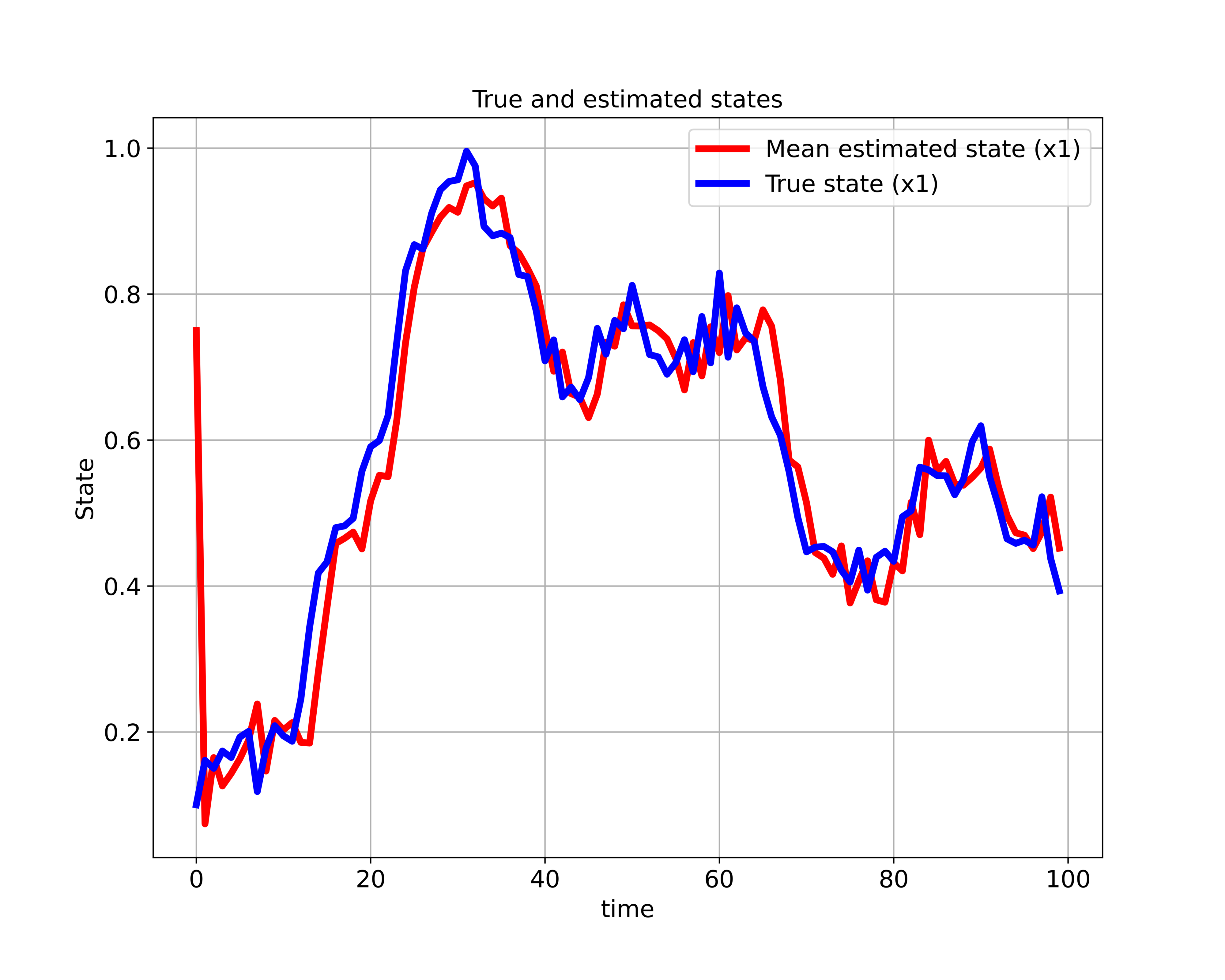
The mean trajectory is computed by using the computed weights and states. Namely, the mean is approximated by using the estimated posterior weight as follows:

(29) $\begin{align*}E[\mathbf{x}_{k}|\mathbf{y}_{0:k},\mathbf{u}_{0:k-1}]=\sum_{i=1}^{N}w^{(i)}_{k}\mathbf{x}_{k}^{(i)}\end{align*}$

We can also use a similar principle to compute any statistics involving the posterior distribution, for more details see the first tutorial part given here. After we compute the mean of estimated state trajectory, we plot the results. The results are given in the two figures below.

Figure 1: “True” and “estimated” state $x_{1}$ of the state space model.

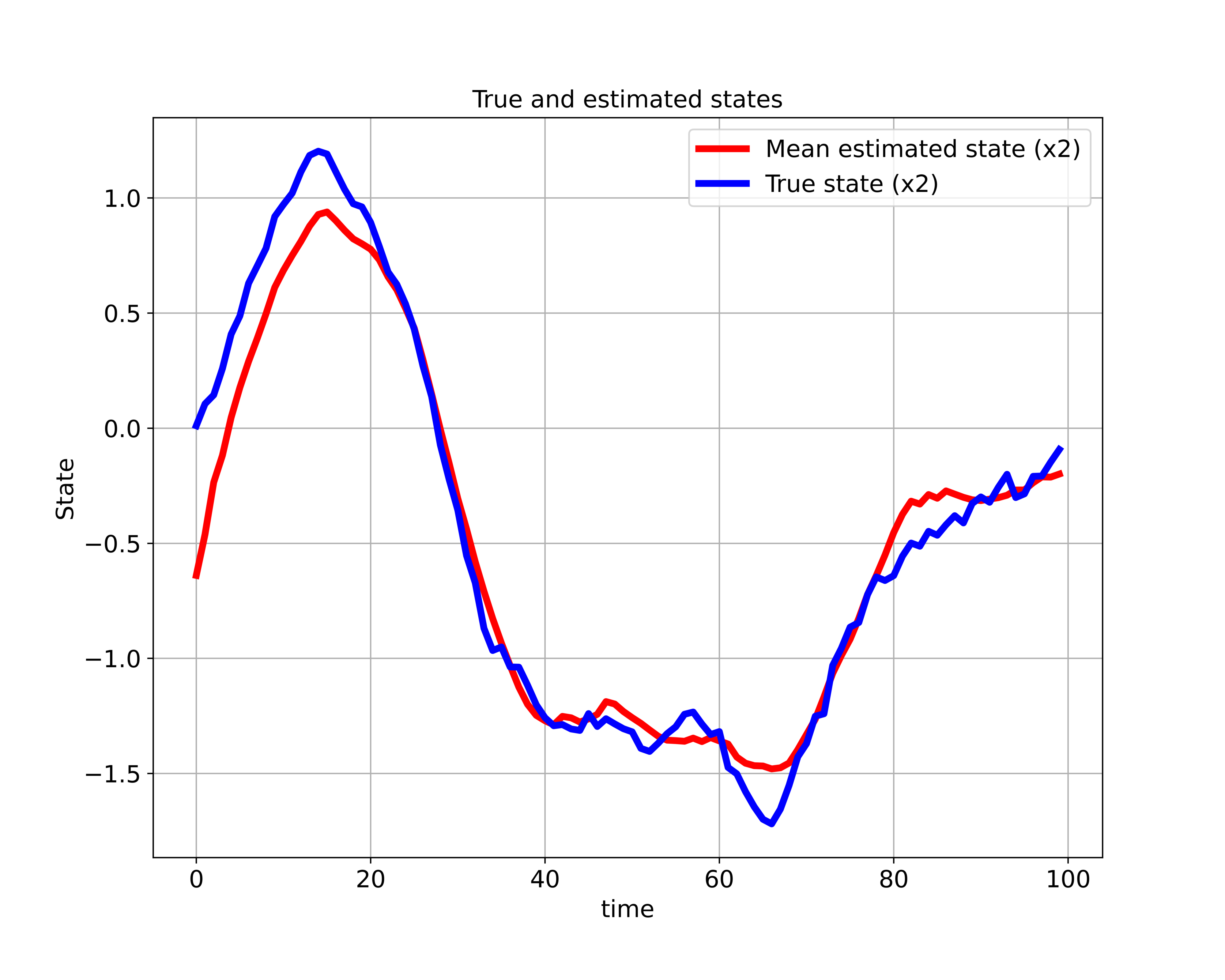Figure 2: “True” and “estimated” state $x_{2}$ of the state space model.

Fig 1. above shows the “true” and “estimated” state $x_{1}$ of the state space model. Fig. 2. shows the “true” and “estimated” state $x_{2}$ of the state space model. We can observe that the mean trajectory computed by the particle filter quickly converges to the true state.

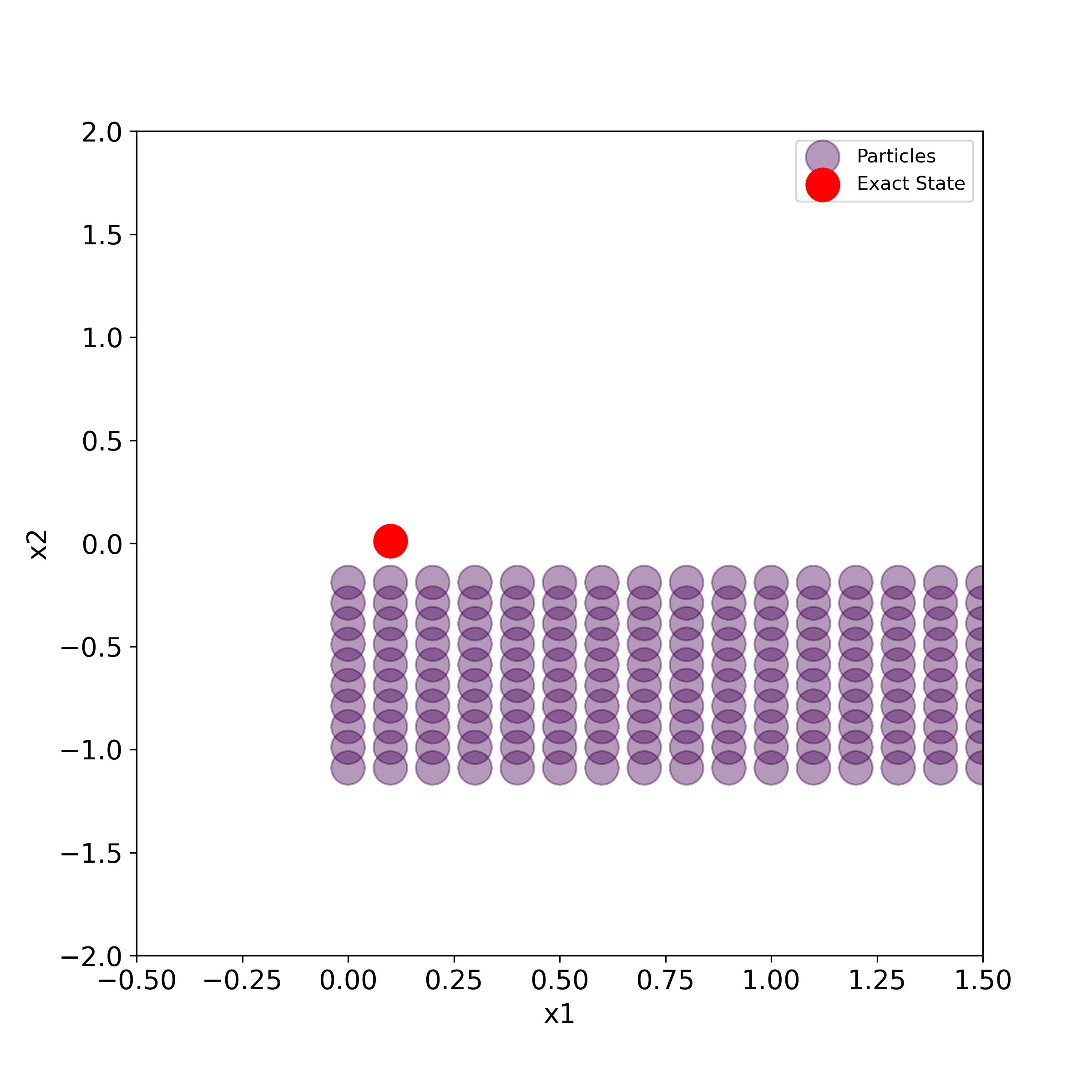
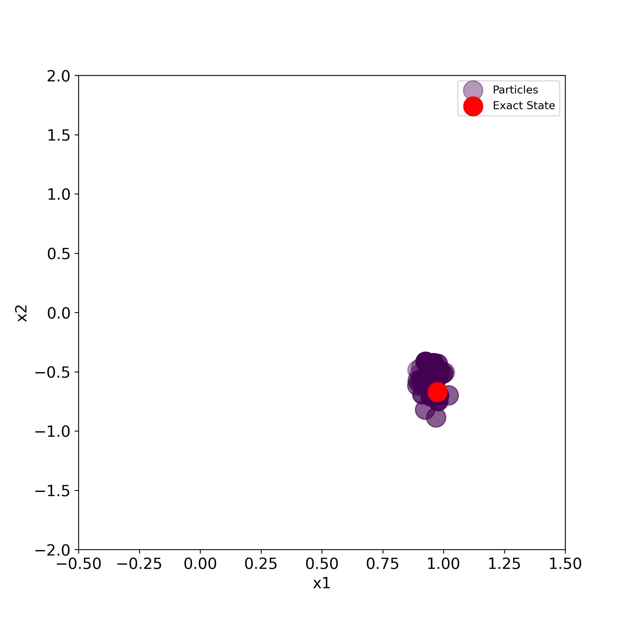
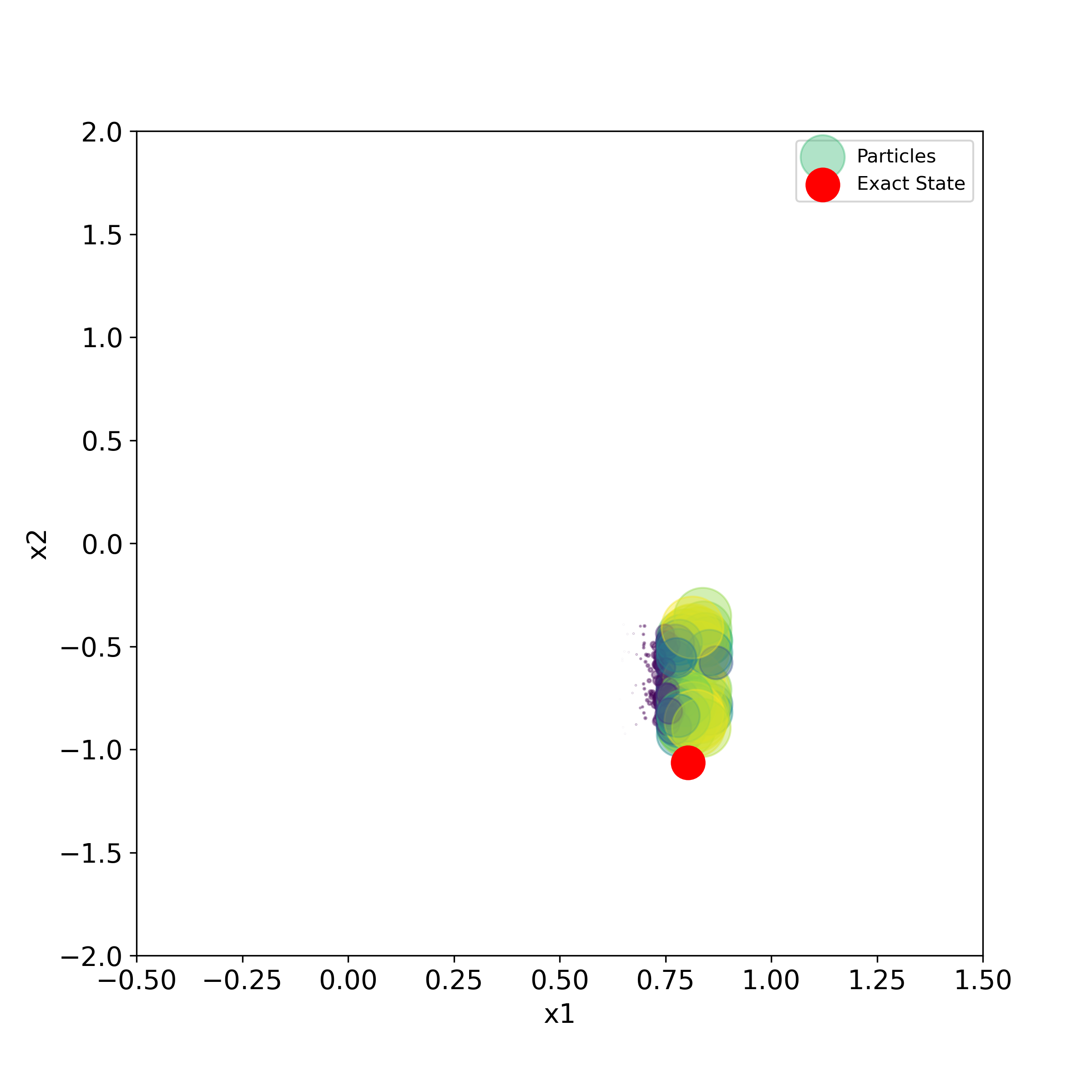
The script given below is used to generate the particles and the true state in the two-dimensional state-space plane.



# use this to generate a series of PNG images for creating the animation
for i in range(numberIterations):
    print(i)
    plt.figure(figsize=(8,8))
    plt.scatter(stateList[i][0,:], stateList[i][1,:], s=50000*weightList[i][0,:],label='Particles', 
                c=weightList[i][0,:], cmap='viridis', alpha =0.4)
    plt.scatter(stateTrajectory[0,i], stateTrajectory[1,i], s=300,c='r', marker='o',label='Exact State' )
    plt.xlim((-0.5,1.5))
    plt.ylim((-2,2))
    plt.xlabel('x1', fontsize=14)
    plt.ylabel('x2',fontsize=14)
    plt.tick_params(axis='both',which='major',labelsize=14)
    plt.legend()
    filename='particles'+str(i).zfill(4)+'.png'
    #time.sleep(0.1)
    plt.savefig(filename,dpi=300)
    #plt.show()

This script will generate a series of PNG images that can be merged together to create animation. We can use Blender (software for creating animations) to create the animation. This is explained in the video tutorial given here.

The generated images are given below.

Brief Summary of Particle Filter Algorithm

Python Implementation of Particle Filter Algorithm

Resampling Methods

Test System

Python Implementation of Particle Filter

admin

You might also like

Design and Test Observers of Dynamical Systems in MATLAB

How To Approximate Expectations and Integrals of Functions by Using the Monte Carlo Method

Control Systems Lecture: Simulation of linear ordinary differential equations using Python and state-space modeling