How To Properly Simulate a Stochastic (Random) Linear State-Space Model in Python – Fusion of Engineering, Control, Coding, Machine Learning, and Science

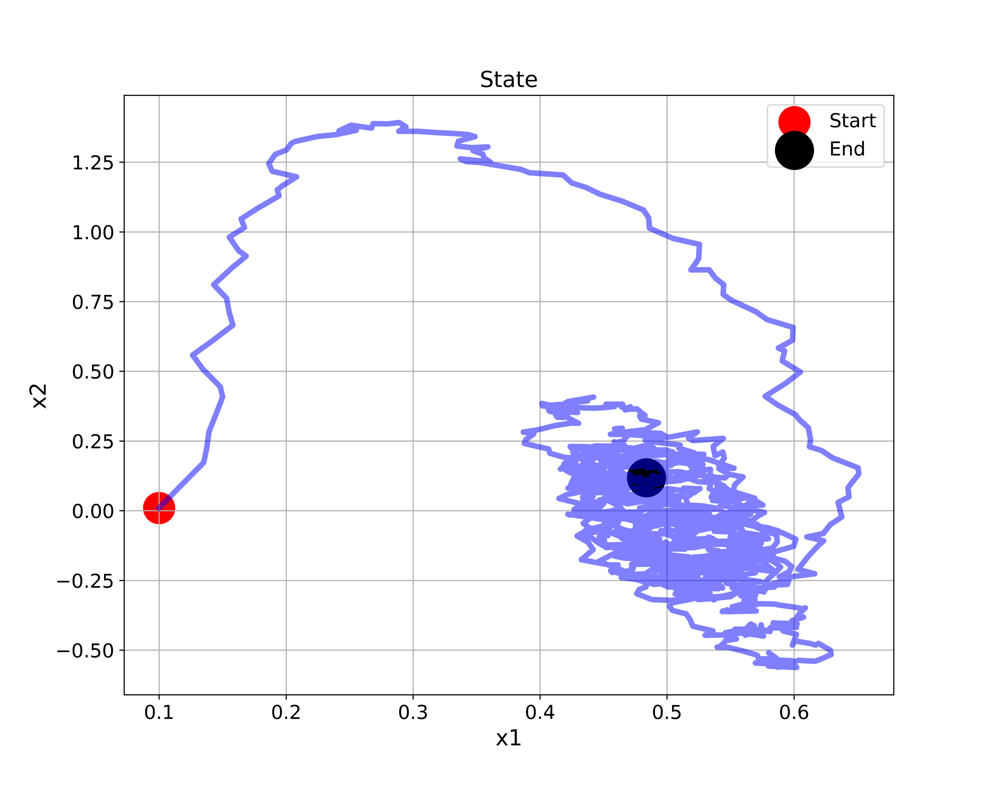
In this control engineering, estimation, and control theory tutorial, we explain how to properly simulate a stochastic (random) linear state-space model in Python. This problem is important for simulating state-space trajectories of dynamical systems that are under the influence of process disturbance and measurement noise. Also, this problem is important for developing and simulating the behavior of stochastic state estimators, such as Kalman filters, particle filters, etc. By the end of this tutorial, you will be able to simulate a stochastic state-space trajectory shown in the figure below.

The YouTube video accompanying this tutorial is given below.

How to Simulate Random or Stochastic State-Space Models in Python

We consider a linear stochastic state-space model

(1) $\begin{align*}\mathbf{x}_{k}& =A\mathbf{x}_{k-1}+B\mathbf{u}_{k-1}+\mathbf{w}_{k-1} \\\mathbf{y}_{k}& =C\mathbf{x}_{k}+\mathbf{v}_{k}\end{align*}$

where

$\mathbf{x}_{k}\in \mathbb{R}^{n}$ is the state vector at the (discrete) time step $k$ .
$\mathbf{u}_{k-1}\in \mathbb{R}^{m_{1}}$ is the control input vector at the time step $k-1$ .
$\mathbf{w}_{k-1}\in \mathbb{R}^{m_{2}}$ is the process disturbance vector (process noise vector) at the time step $k-1$ .
$\mathbf{y}_{k}\in \mathbb{R}^{r}$ is the observed output vector at the time step $k$ .
$\mathbf{v}_{k}\in \mathbb{R}^{r}$ is the measurement noise vector at the discrete time step $k$ .
$A\in \mathbb{R}^{n\times n},B\in \mathbb{R}^{n\times m}$ and $C\in \mathbb{R}^{r\times n}$ are system matrices.

Here, we assume that the random vectors $\mathbf{w}_{k}$ and $\mathbf{v}_{k}$ are distributed according to some prescribed distributions. In this tutorial, for simplicity, we assume that both of these vectors are normally distributed with given mean vectors and covariance matrices. However, everything explained in this tutorial can be generalized to random vectors with arbitrary distributions.

Let the mean vector and the covariance matrix of $\mathbf{w}_{k}$ be denoted by $\mu_{w}$ and $Q_{w}$ , respectively. Similarly, let the mean vector and the covariance matrix of $\mathbf{v}_{k}$ be denoted by $\mu_{v}$ and $Q_{v}$ , respectively. By using the mathematical notation, we can write

(2) $\begin{align*}\mathbf{w}_{k} \sim \mathcal{N}(\mu_{w}, Q_{w}),\;\; \mathbf{v}_{k} \sim \mathcal{N}(\mu_{v}, Q_{v})\end{align*}$

where $\mathcal{N}(\cdot, \cdot )$ is the mathematical notation for the normal distribution. The first entry in this notation is the mean vector and the second entry is the covariance matrix. The symbol “ $\sim$ ” means that the vector on the left side of this symbol is distributed according to the distribution on the right side of the symbol.

Our goal is to simulate the state-space model (1) starting from some initial state $\mathbf{x}_{0}$ and for user-defined control inputs. That is, our goal is to simulate a sequence of states and outputs:

(3) $\begin{align*}\mathbf{x}_{1},\mathbf{x}_{2},\mathbf{x}_{3},\ldots, \mathbf{x}_{N} \\\mathbf{y}_{1},\mathbf{y}_{2},\mathbf{y}_{3},\ldots, \mathbf{y}_{N} \end{align*}$

To explain how to simulate a state-space model in Python, we use a second-order mass-spring-damper system originally introduced in our previous tutorial. The model is described as a continuous-time state-space model:

(4) $\begin{align*}\dot{\mathbf{x}} & =A\mathbf{x}+B\mathbf{u} \\\mathbf{y}& =C\mathbf{x}\end{align*}$

where

(5) $\begin{align*}A=\begin{bmatrix} 0 & 1 \\ -\frac{k_{s}}{m} & -\frac{k_{d}}{m} \end{bmatrix},\;\; B=\begin{bmatrix} 0 \\ \frac{1}{m} \end{bmatrix},\;\; C=\begin{bmatrix} 1 & 0 \end{bmatrix}\end{align*}$

where $k_{s}$ is the spring constant, $k_{d}$ is the damper constant, and $m$ is the mass. The state-space vector is

(6) $\begin{align*}\mathbf{x}=\begin{bmatrix} x_{1} \\ x_{2} \end{bmatrix}\end{align*}$

where $x_{1}$ is the position of the mass, and $x_{2}$ is the velocity of the mass. The first step is to discretize the state-space model. To discretize the state-space model, we use the backward Euler method. The backward Euler method approximates the state derivative by using the backward finite difference discretization:

(7) $\begin{align*}\dot{\mathbf{x}} \approx \frac{\mathbf{x}_{k}-\mathbf{x}_{k-1}}{h}\end{align*}$

where $\mathbf{x}(kh): =\mathbf{x}_{k}$ , and $h$ is a sufficiently small discretization time step. By substituting (7) in the state equation of (4), we obtain

(8) $\begin{align*}\frac{\mathbf{x}_{k}-\mathbf{x}_{k-1}}{h} & \approx A\mathbf{x}_{k}+B\mathbf{u}_{k} \\\mathbf{x}_{k}-\mathbf{x}_{k-1} & \approx hA\mathbf{x}_{k}+hB\mathbf{u}_{k} \\\mathbf{x}_{k}-hA\mathbf{x}_{k} & \approx \mathbf{x}_{k-1}+hB\mathbf{u}_{k} \\(I-hA)\mathbf{x}_{k} & \approx \mathbf{x}_{k-1}+hB\mathbf{u}_{k} \\\mathbf{x}_{k} & \approx (I-hA)^{-1}\mathbf{x}_{k-1}+h(I-hA)^{-1}B\mathbf{u}_{k} \end{align*}$

By replacing the approximation symbol with an equality symbol, and by replacing $\mathbf{u}_{k}$ with $\mathbf{u}_{k-1}$ , we obtain the discretized state equation

(9) $\begin{align*}\mathbf{x}_{k} = A_{D}\mathbf{x}_{k-1}+B_{D}\mathbf{u}_{k-1} \end{align*}$

where

(10) $\begin{align*}A_{D}=(I-hA)^{-1},\;\; B_{D}=h(I-hA)^{-1}B\end{align*}$

The replacement of $\mathbf{u}_{k}$ by its delayed version $\mathbf{u}_{k-1}$ does not change anything qualitatively about our state-space model. The output equation is

(11) $\begin{align*}\mathbf{y}_{k}=C\mathbf{x}_{k}\end{align*}$

Before we explain the Python script for simulating the state-space model, we need to explain why we used the backward Euler method. Namely, we can also approximate the first derivative of the state by using forward difference discretization:

(12) $\begin{align*}\dot{\mathbf{x}} \approx \frac{\mathbf{x}_{k+1}-\mathbf{x}_{k}}{h}\end{align*}$

and by substituting this equation in the state-space model (4), we obtain

(13) $\begin{align*}& \frac{\mathbf{x}_{k+1}-\mathbf{x}_{k}}{h} =A\mathbf{x}_{k}+B\mathbf{u}_{k} \\& \mathbf{x}_{k+1}=(I+hA)\mathbf{x}_{k}+hB\mathbf{u}_{k}\end{align*}$

The resulting discrete-time state-space model might not be stable. On the other hand, the discrete-time state-space model obtained by using the backward Euler discretization has much better stability properties than the discrete-time state-space model obtained by using the forward Euler method.

Also, here we have to emphasize that we discretized the continuous-time model that is not affected by the measurement and process noise. Later on, we add the process and measurement noise to the discrete-time model. On the other hand, if we would start from the continuous-time model that is affected by the continuous-time measurement and process noise, then the discretization procedure would be much more complex.

Next, we explain the Python script for simulating the state-space model. First, we import the necessary libraries and define the mean vectors and covariance matrices of the process disturbance and measurement noise distributions.


import numpy as np
import matplotlib.pyplot as plt
from scipy.stats import multivariate_normal


# process disturbance
# mean
mP=np.array([0,0])
# covariance
cP=np.array([[0.0001, 0],[0, 0.0001]])

# measurement noise
# mean
mN=np.array([0])
# covariance
cN=np.array([[0.001]])


# create distributions 
# process disturbance distribution
pDistribution=multivariate_normal(mean=mP,cov=cP)
# noise distribution
nDistribution=multivariate_normal(mean=mN,cov=cN)

To create the distributions, we use the Python library called SciPy and its Stats module. The Stats module implements a number of functions for performing probability and statistics calculations in Python. To create the distributions, we use the function “multivariate_normal”. The first input of this function is the mean vector and the second input is the covariance matrix. Once we define the distributions, we can draw the samples like this

pDistribution.rvs(size=1).reshape(2,1)

The result is a sample of the process disturbance

array([[-0.03230093],
       [-0.00844334]])

By using the same principle you can generate samples from other distributions. For more details, see the Stats module reference page given here. After this, we define the model and perform discretization:


# measurement noise
# mean
mN=np.array([0])
# covariance
cN=np.array([[0.001]])


# create distributions 
# process disturbance distribution
pDistribution=multivariate_normal(mean=mP,cov=cP)
# noise distribution
nDistribution=multivariate_normal(mean=mN,cov=cN)


# Construct a continuous-time system
m=5
ks=200
kd=30

Ac=np.array([[0,1],[-ks/m, -kd/m]])
Cc=np.array([[1,0]])
Bc=np.array([[0],[1/m]])

# discretize the system
# discretization constant
h=0.005

A=np.linalg.inv(np.eye(2)-h*Ac)
B=h*np.matmul(A,Bc)
C=Cc

The Python script given below is used to simulate the state-space model:

# select the initial state
x0=np.array([[0.1],[0.01]])

# control input
#controlInput=10*np.random.rand(1,simTime)
cI=100*np.ones((1,simSteps))

# zero-state trajectory
sT=np.zeros(shape=(2,simSteps+1))

# output 
output=np.zeros(shape=(1,simSteps))

# set the initial state
sT[:,[0]]=x0

# simulate the state-space model
for i in range(simSteps):
    sT[:,[i+1]]=np.matmul(A,sT[:,[i]])+np.matmul(B,cI[:,[i]])+pDistribution.rvs(size=1).reshape(2,1)
    output[:,[i]]=np.matmul(C,sT[:,[i]])+nDistribution.rvs(size=1).reshape(1,1)

First, we define the initial state and the control input sequence. Then, we define empty arrays for storing the simulated state and output sequences. Finally, we use a simple for loop to simulate the discrete-time system. In every step of the loop we generate random samples of the process disturbance and measurement noise.

The script given below is used to plot the simulation results.

# create a time vector
timeVector=np.linspace(0,(simSteps-1)*h,simSteps)

# plot the time response
plt.figure(figsize=(10,8))
plt.plot(timeVector,sT[0,0:simSteps], color='blue',linewidth=4)
plt.title("State", fontsize=14)
plt.xlabel("time", fontsize=14)
plt.ylabel("State",fontsize=14)
plt.tick_params(axis='both',which='major',labelsize=14)
plt.grid(visible=True)
plt.savefig("stateTrajectoryTime.png",dpi=600)
plt.show()

# plot the state-space trajectory
plt.figure(figsize=(10,8))
plt.plot(sT[0,0:simSteps],sT[1,0:simSteps], color='blue',linewidth=4,alpha=0.5)
plt.title("State", fontsize=16)
plt.xlabel("x1", fontsize=16)
plt.ylabel("x2",fontsize=16)
plt.tick_params(axis='both',which='major',labelsize=14)
plt.grid(visible=True)
plt.scatter(sT[0,0], sT[1,0], s=500,c='r', marker='o',label='Start' )
plt.scatter(sT[0,-1], sT[1,-1], s=500,c='k', marker='o',linewidth=6,label='End' )
plt.legend(fontsize=14)
plt.savefig("stateTrajectory.png",dpi=600)
plt.show()

The time response of the first state is given in the figure below.

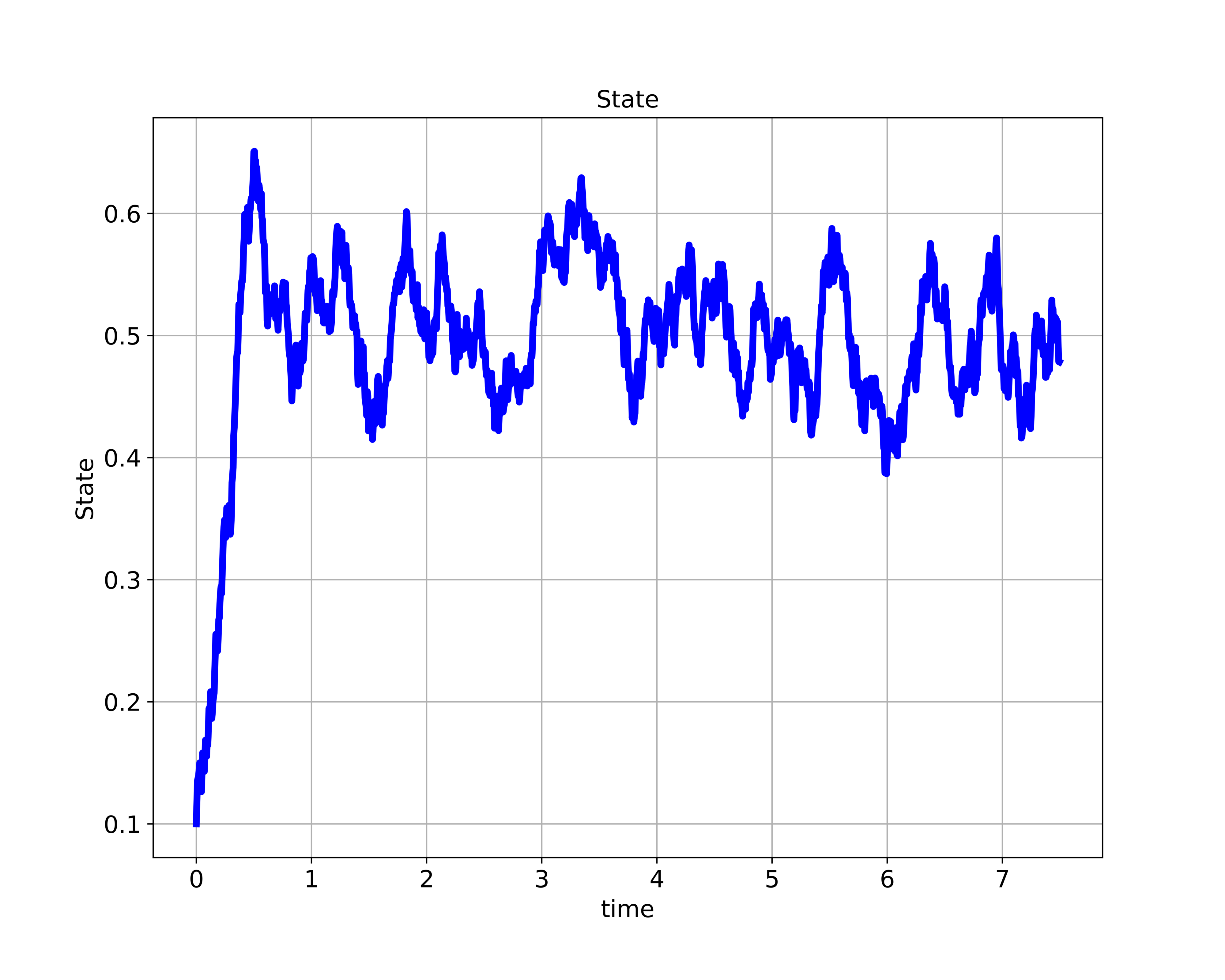Figure 1: Simulated state $x_{1}$ as a function of time.

The complete state-space trajectory is given in the figure below.

How to Simulate Random or Stochastic State-Space Models in Python

admin

You might also like

Design and Test Observers of Dynamical Systems in MATLAB

How to Install ROS2 Humble Hawksbill in Ubuntu 22.04 and How to Run a Hello World Example

Clear and Detailed Explanation of Kinematics, Equations, and Geometry of Motion of Differential Wheeled Robot (Differential Drive Robot)