Clear and Detailed Explanation of Kinematics, Equations, and Geometry of Motion of Differential Wheeled Robot (Differential Drive Robot) – Fusion of Engineering, Control, Coding, Machine Learning, and Science

In this robotics tutorial, we explain the kinematics, equations, and geometry of motion of a differential wheeled robot. The differential wheeled robot is also known as the differential drive robot. We will derive the equations describing the kinematics of the robot, and in the second part of this tutorial, we will explain how to simulate the motion of the differential wheeled robot in Python. The YouTube tutorial accompanying this post is given below.

Basic Description of the Differential Drive Robot and Motion Modes

The videos given below show a real-life differential wheeled robot and its motion.

The photograph of the differential drive robot is given below.

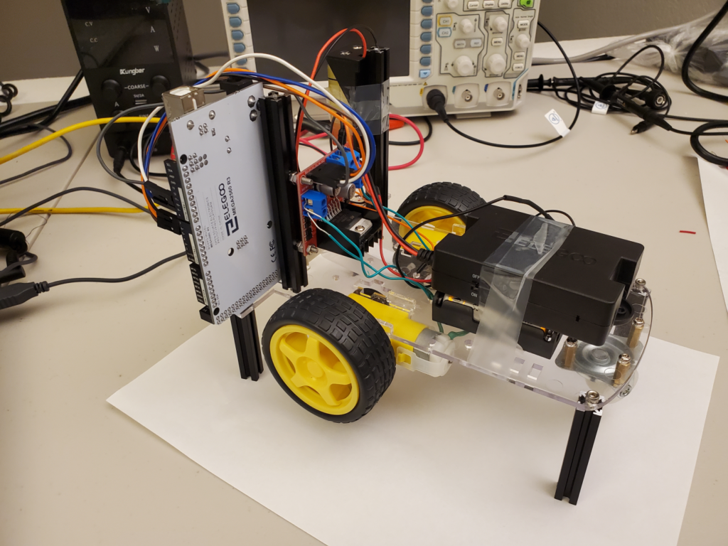
Figure 1: Real-life differential drive robot.

The robot consists of two wheels that are driven by two DC motors, and the caster wheel. The caster wheel is a passive wheel that provides support and two rotations. These two rotations enable the robot to move in any direction.

The figure given below shows a top view of the differential drive robot after a few geometrical simplifications that do not affect the modeling generality.

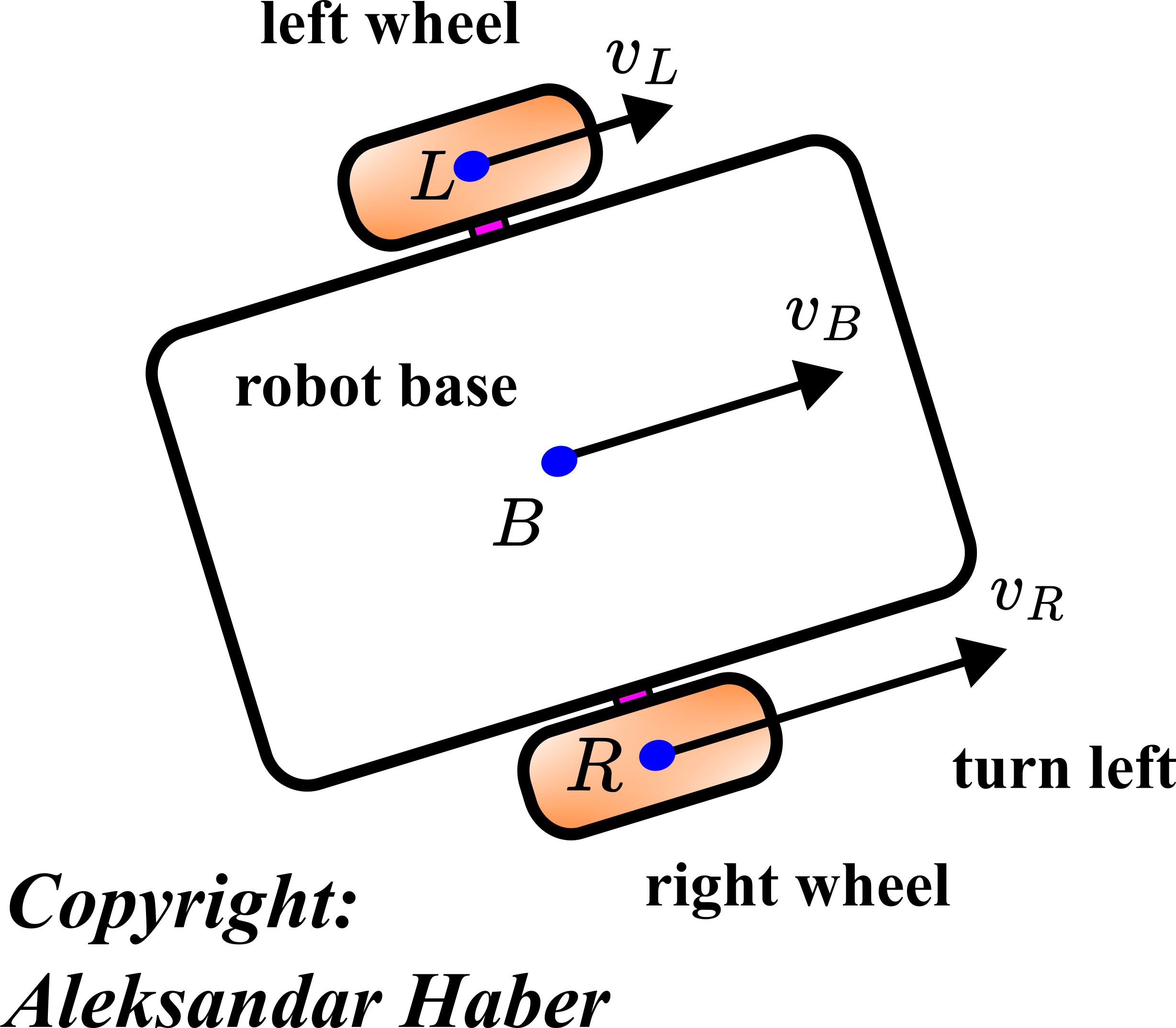
Figure 2: Top view of the differential drive robot. In this scenario, the robot is turning left.

The robot consists of the robot base and two wheels. The points $L$ and $R$ are located at the corresponding centers of the two wheels. The point $B$ is the point in the middle of the line connecting the points $L$ and $R$ . The velocity $v_{L}$ is the velocity of the center point of the left wheel. Similarly, the velocity $v_{R}$ is the velocity of the center point of the right wheel. These velocities are a direct consequence of the fact that the wheels are spinning due to the torques exerted by the motors. In the figure shown above, the robot is turning left. This is because the intensity of the velocity $v_{R}$ is larger than the intensity of the velocity $v_{L}$ . In fact, as we will be shown later, in this configuration, all the 3 points $L$ , $B$ , and $R$ will describe concentric circles centered at the instantaneous center of rotation (this point is also known as the instant center of rotation or instantaneous velocity center).

Here, it is very important to emphasize the following:

We can completely control the robot’s motion by controlling the right and left wheel angular velocities or the right and left wheel rotational angles. The velocities $v_{L}$ and $v_{R}$ are linearly proportional to the angular velocities of the right and left wheels.

Let us illustrate this further with several control scenarios.

The figure below illustrates how we can achieve the straight motion of the robot.

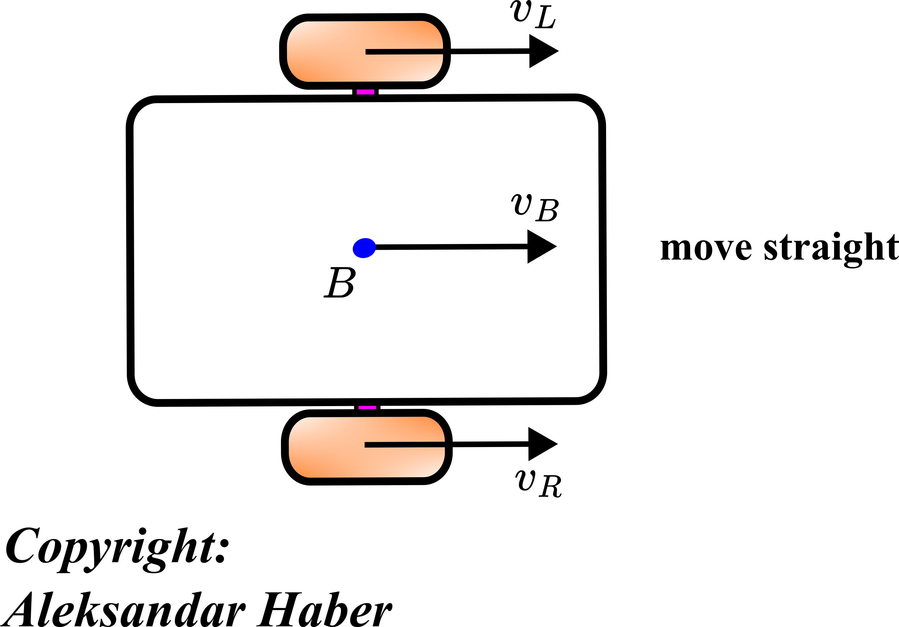
Figure 3: Top view of the differential drive robot. In this scenario, the robot is moving straight.

In the scenario shown in the figure above, the robot is moving straight. This is because the intensities of the velocities $v_{L}$ and $v_{R}$ are equal. Consequently, the instantaneous center of rotation is at infinity and all the points describe straight lines.

The figure below shows another important scenario.

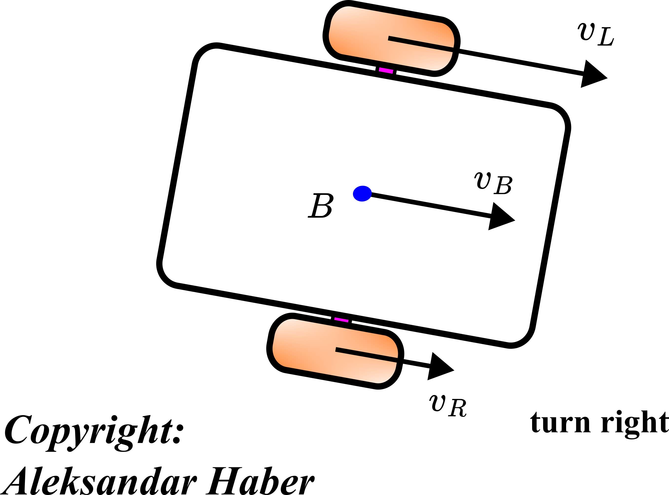
Figure 4: Top view of the differential drive robot. In this scenario, the robot is moving right.

The robot is moving right. This is because the intensity of the velocity $v_{L}$ is larger than the intensity of the velocity of $v_{R}$ .

The figure below shows the final scenario.

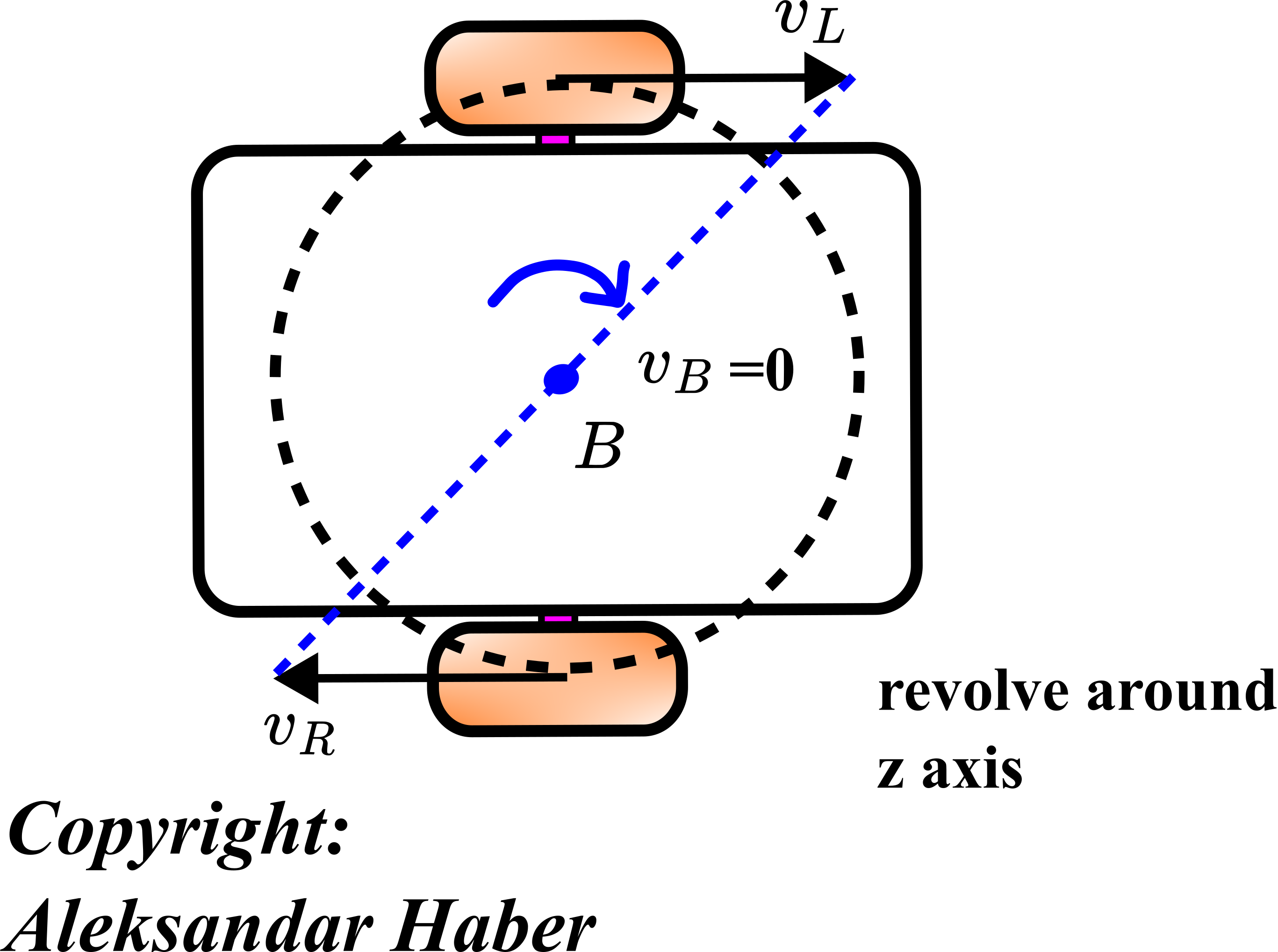Figure 5: Top view of the differential drive robot. In this scenario, the robot is rotating around the point $B$ .

In the scenario shown in the figure above, the robot is rotating around the point $B$ . This is the point at the middle of the line connecting the centers of left and right wheels. The rotation is due to the fact that the velocities have identical intensities and opposite directions.

To conclude:

By changing the velocities of the centers of two wheels, or equivalently, by changing the angular velocities of the two wheels, we can control the robot’s motion.

Detailed Kinematic Analysis of Differential Drive Robot

Here, we provide a detailed kinematic analysis of the differential drive robot. We want to establish the equations that will relate the angular velocities of two wheels with the velocity of the center of the robot, and the angular velocity of robot rotation. In the next tutorial, we will solve the direct and inverse kinematic problem, that will establish a relationship between the position of the robot’s with the angles of rotation of two wheels.

The figure given below shows the kinematic diagram of the robot.

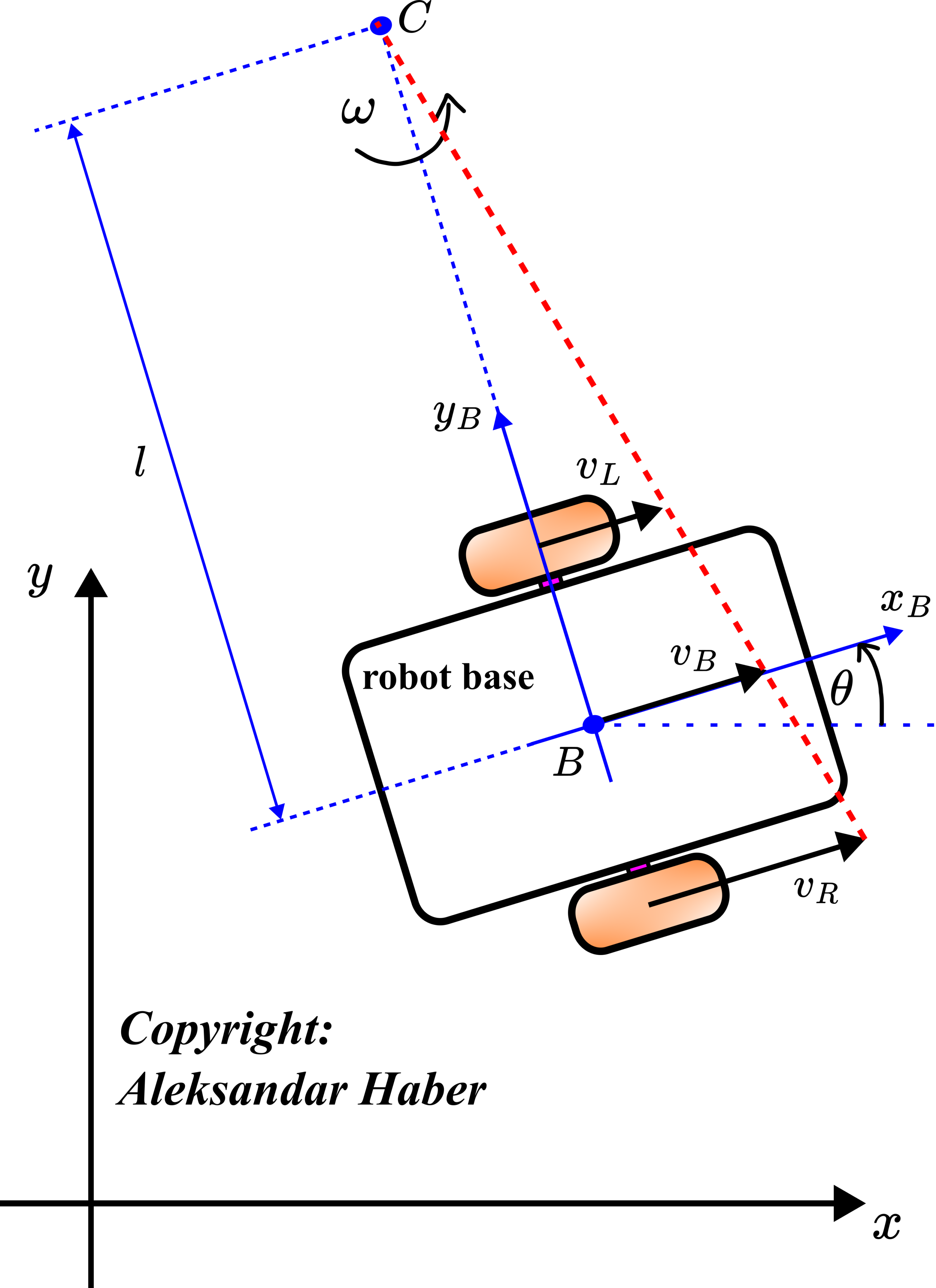
Figure 6: Kinetic (velocity) diagram of the differential drive robot.

The coordinate system $x-y$ is a fixed (inertial) coordinate system. The coordinate system $x_{B}-y_{B}$ with the center at the point $B$ is the coordinate system rigidly attached to the robot body. It translates and rotates together with the robot. The coordinate system $x_{B}-y_{B}$ is called the body coordinate system or the body frame (in robotics, coordinate systems are also called frames).

The point $C$ is the instantaneous center of rotation of the robot. From the velocity analysis perspective, during a short time interval, the robot seems to rotate around the instantaneous center of rotation. This point is constructed by finding an intersection of the line connecting the top of the velocity arrows with the line passing through the centers of the wheels. The symbol $\omega$ denotes the instantaneous angular velocity.

The angle $\theta$ is the rotation angle of the robot body. This angle is at the same time the rotation of the body frame with respect to the inertial frame $x-y$ .

Under the assumption that the intensities of the velocities are not changing during a time interval, the points $L$ , $B$ , and $R$ describe concentric circles centered at the point $C$ during the considered time interval. This is shown in the figure below.

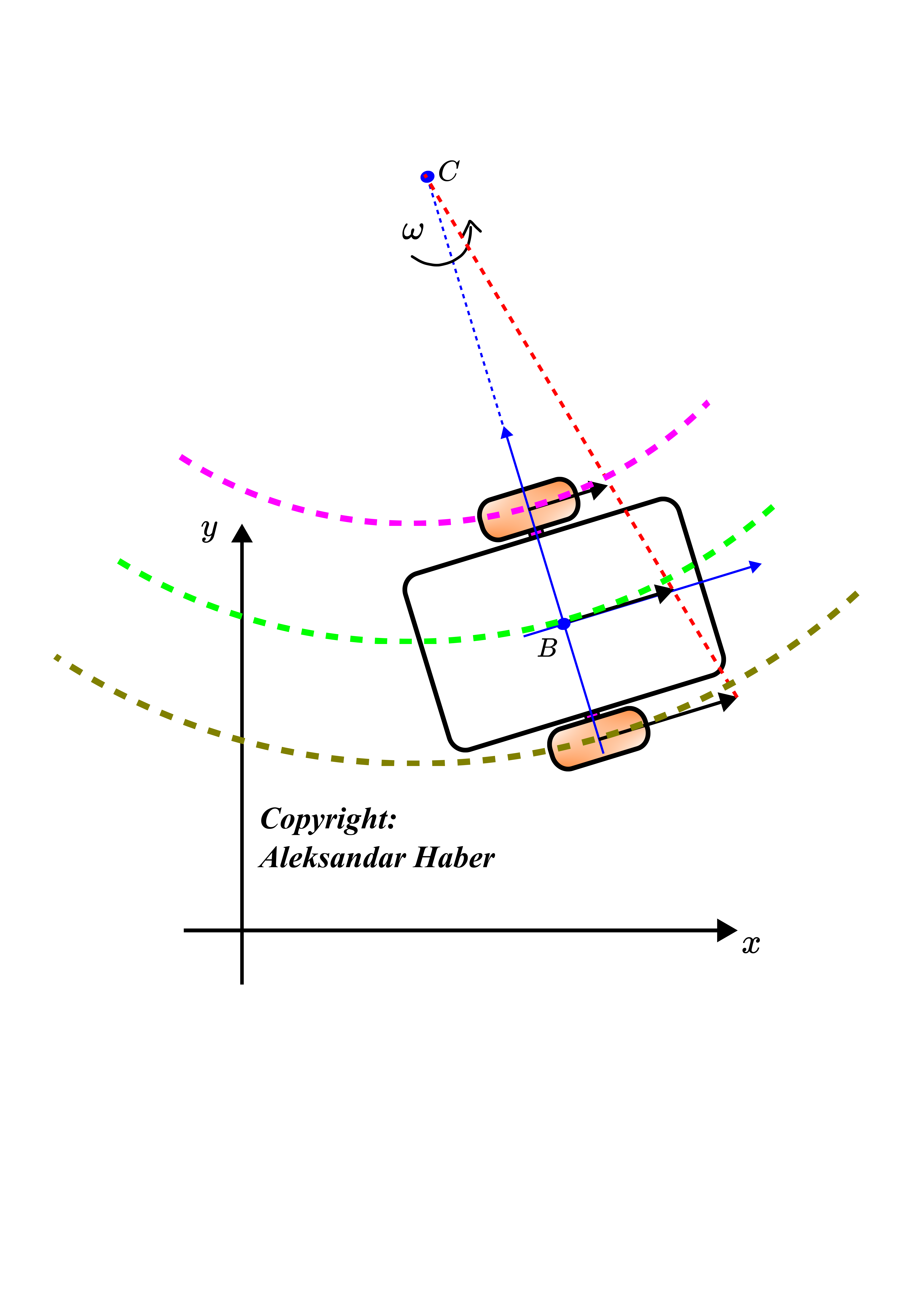Figure 7: Trajectories described by the points $L$ , $B$ , and $R$ during a time interval.

The graph given below shows all the dimensions of the robot that are necessary for developing the kinematic equations.

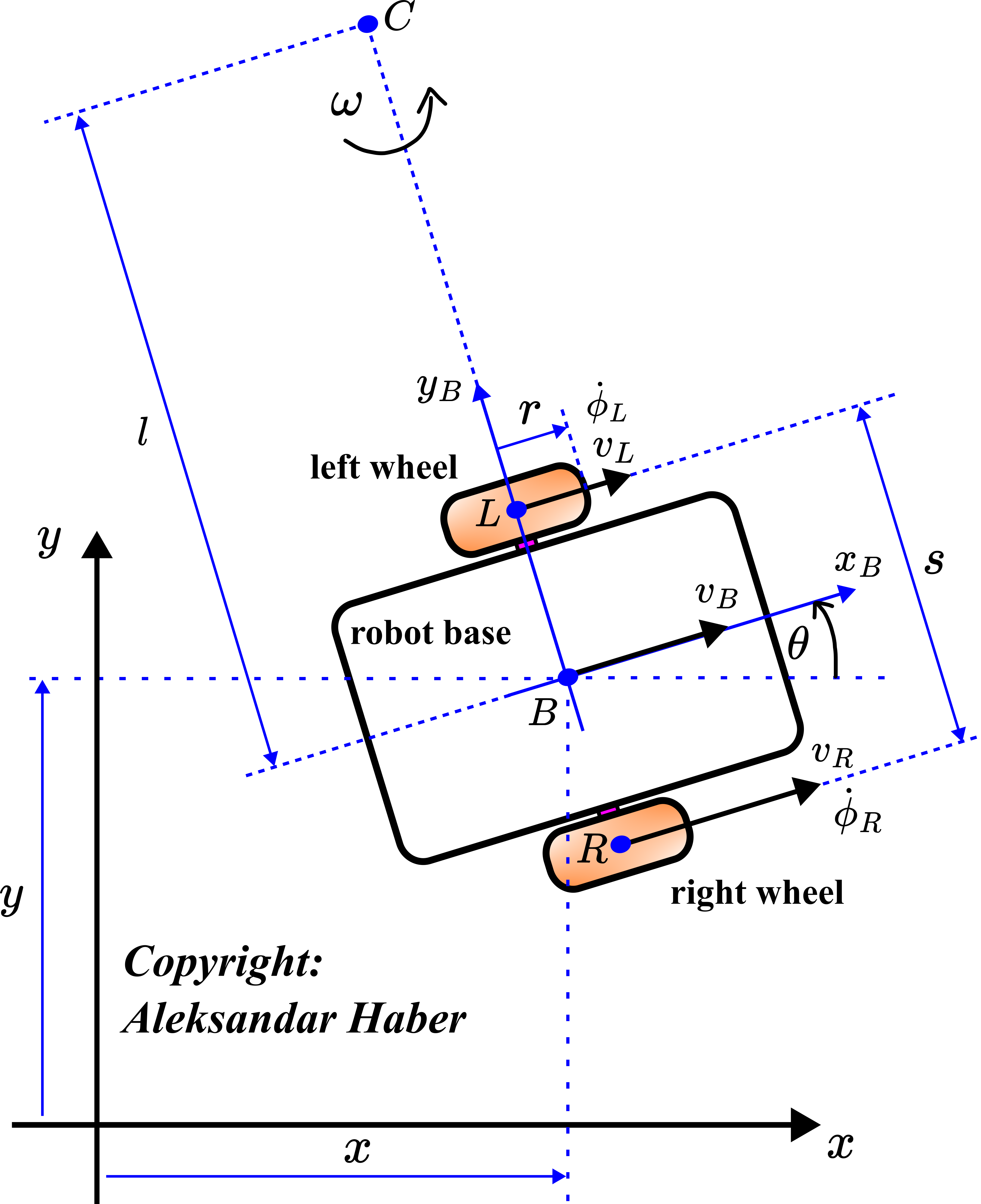
Figure 8: Detailed kinematic diagram with all the parameters.

Here, for clarity of this lecture, we will summarize once more all the involved quantities

$x$ and $y$ are the translation coordinates of the body frame attached to the point $B$ with respect to the inertial frame $x-y$ .
$\theta$ is the angle of rotation of the robot which is at the same time the angle between the body frame and the inertial frame.
$x_{B}$ and $y_{B}$ are the coordinates in the body frame and at the same time they denote the axes of the body frame.
$C$ is the instantaneous center of rotation.
$\omega$ is the instantaneous angular velocity of the robot body.
$L$ is the center point of the left wheel.
$R$ is the center point of the right wheel.
$B$ is the middle point between the points $L$ and $R$ .
$v_{L}$ is the velocity of the center of the left wheel.
$v_{R}$ is the velocity of the center of the right wheel.
$v_{B}$ is the velocity of the point $B$ .
$\dot{\phi}_{L}$ is the angular velocity of the left wheel.
$\dot{\phi}_{R}$ is the angular velocity of the right wheel.
$l$ is the distance between the point $B$ and the point $C$ .
$r$ is the radius of the wheels.
$s$ is the distance between the points $L$ and $R$ .
$\dot{x}$ is the projection of the velocity $v_{B}$ on the $x$ axis.
$\dot{y}$ is the projection of the velocity $v_{B}$ on the $y$ axis.

In the sequel, we will derive the equations that will relate $\dot{\phi}_{L}$ and $\dot{\phi}_{R}$ with $\dot{x}$ , $\dot{y}$ , and $\dot{\theta}$ . These equations will enable us to predict the robot center point velocity and angular velocity as the function of control variables $\dot{\phi}_{L}$ and $\dot{\phi}_{R}$ .

That is, we start from the assumption that the following quantities and parameters are known $\dot{\phi}_{L}$ , $\dot{\phi}_{R}$ , $s$ , and $r$ , and we want to determine $\dot{x}$ , $\dot{y}$ , and $\dot{\theta}$ .

From Fig. 8, we have

(1) $\begin{align*}v_{L}=\omega (l-\frac{s}{2}) \\v_{R}=\omega (l+\frac{s}{2})\end{align*}$

The issue with these two equations is that both $l$ and $\omega$ are not known. Consequently, we need to solve these two equations for $l$ and $\omega$ . From the first equation in (1), we can express the variable $\omega$ as follows

(2) $\begin{align*}\omega=\frac{v_{L}}{l-\frac{s}{2}}\end{align*}$

By substituting this equation in the first equation of (1), we obtain

(3) $\begin{align*}v_{R}&=\frac{v_{L}}{l-\frac{s}{2}}\big(l+\frac{s}{2} \big) \\v_{R}\big(l-\frac{s}{2} \big)& =v_{L}\big(l+\frac{s}{2} \big) \\v_{R}l-v_{R}\frac{s}{2}&=v_{L}l+v_{L}\frac{s}{2} \\l(v_{R}-v_{L})&=v_{R}\frac{s}{2}+v_{L}\frac{s}{2} \end{align*}$

From the last equation, we obtain

(4) $\begin{align*}l=\frac{s(v_{R}+v_{L})}{2(v_{R}-v_{L})} \end{align*}$

By substituting the last equation in the first equation of (1), we obtain

(5) $\begin{align*}v_{L}&=\omega\big(l-\frac{s}{2} \big) \\v_{L}&=\frac{\omega s}{2}\Big(\frac{v_{R}+v_{L}}{v_{R}-v_{L}} -1 \Big)\\v_{L}&=\frac{\omega s}{2}\Big(\frac{2v_{L}}{v_{R}-v_{L}} \Big)\end{align*}$

From the last equation, we obtain

(6) $\begin{align*}\omega = \frac{v_{R}-v_{L}}{s}\end{align*}$

For clarity, we repeat the expressions for $\omega$ and $l$ :

(7) $\begin{align*}l & =\frac{s(v_{R}+v_{L})}{2(v_{R}-v_{L})} \\\omega & = \frac{v_{R}-v_{L}}{s}\end{align*}$

From Fig. 8, we have

(8) $\begin{align*}\dot{x}=v_{B}\cos(\theta) \\\dot{y}=v_{B}\sin(\theta) \\\dot{\theta}=\omega\end{align*}$

The last set of equations can be written compactly

(9) $\begin{align*}\begin{bmatrix}\dot{x} \\\dot{y} \\\dot{\theta}\end{bmatrix}=\begin{bmatrix}\cos(\theta) & 0 \\ \sin(\theta) & 0 \\ 0 & 1 \end{bmatrix}\begin{bmatrix} v_{B} \\ \omega \end{bmatrix}\end{align*}$

On the other hand, we have that the intensity of the velocity $v_{B}$ is given by

(10) $\begin{align*}v_{B}=\omega \cdot l \end{align*}$

By substituting the expressions for $l$ and $\omega$ given in (7) into the last equation, we obtain

(11) $\begin{align*}v_{B}& =\frac{v_{R}-v_{L}}{s}\cdot \frac{s}{2}\frac{(v_{R}+v_{L})}{(v_{R}-v_{L})} \\v_{B}& = \frac{v_{R}+v_{L}}{2}\end{align*}$

By combining this equation, with the equation for $\omega$ from (7), we obtain the following equations

(12) $\begin{align*}v_{B}& = \frac{v_{R}+v_{L}}{2} \\\omega & = \frac{v_{R}-v_{L}}{s}\end{align*}$

The last two equations can be written compactly

(13) $\begin{align*}\begin{bmatrix} v_{B} \\ \omega \end{bmatrix}= \begin{bmatrix} \frac{1}{2} & \frac{1}{2} \\ -\frac{1}{s} & \frac{1}{s} \end{bmatrix}\begin{bmatrix} v_{L} \\ v_{R} \end{bmatrix}\end{align*}$

By substituting the equation (13) into the equation (9), we obtain

(14) $\begin{align*}\begin{bmatrix}\dot{x} \\\dot{y} \\\dot{\theta}\end{bmatrix} & =\begin{bmatrix}\cos(\theta) & 0 \\ \sin(\theta) & 0 \\ 0 & 1 \end{bmatrix}\begin{bmatrix} \frac{1}{2} & \frac{1}{2} \\ -\frac{1}{s} & \frac{1}{s} \end{bmatrix}\begin{bmatrix} v_{L} \\ v_{R} \end{bmatrix} \\\begin{bmatrix}\dot{x} \\\dot{y} \\\dot{\theta}\end{bmatrix} & =\begin{bmatrix}\frac{\cos(\theta)}{2} & \frac{\cos(\theta)}{2} \\ \frac{\sin(\theta)}{2} & \frac{\sin(\theta)}{2} \\ -\frac{1}{s} & \frac{1}{s} \end{bmatrix}\begin{bmatrix} v_{L} \\ v_{R} \end{bmatrix}\end{align*}$

The last system of equations can be expanded as follows

(15) $\begin{align*}\dot{x}& =\frac{v_{L}}{2}\cos(\theta)+\frac{v_{R}}{2}\cos(\theta) \\\dot{y}& =\frac{v_{L}}{2}\sin(\theta)+\frac{v_{R}}{2}\sin(\theta) \\\dot{\theta} & = -\frac{1}{s}v_{L}+ \frac{1}{s}v_{R}\end{align*}$

The system of equations (15) relates the controlled wheel velocities $v_{R}$ and $v_{L}$ with the velocity projections of the center $B$ of the robot and the angular velocity of the robot. However, we know that the wheel velocities are actually functions of the wheel angular velocities $\dot{\phi}_{L}$ and $\dot{\phi}_{R}$ :

(16) $\begin{align*}v_{L}=r \dot{\phi}_{L} \\v_{R}=r \dot{\phi}_{R}\end{align*}$

The last two equations can be compactly written in the vector-matrix form

(17) $\begin{align*}\begin{bmatrix}v_{L} \\ v_{R} \end{bmatrix}= \begin{bmatrix} r & 0 \\ 0 & r \end{bmatrix}\begin{bmatrix} \dot{\phi}_{L} \\ \dot{\phi}_{R} \end{bmatrix}\end{align*}$

By substituting (17) in (14), we obtain

(18) $\begin{align*}\begin{bmatrix}\dot{x} \\\dot{y} \\\dot{\theta}\end{bmatrix} & =\begin{bmatrix}\frac{\cos(\theta)}{2} & \frac{\cos(\theta)}{2} \\ \frac{\sin(\theta)}{2} & \frac{\sin(\theta)}{2} \\ -\frac{1}{s} & \frac{1}{s} \end{bmatrix}\begin{bmatrix} r & 0 \\ 0 & r \end{bmatrix}\begin{bmatrix} \dot{\phi}_{L} \\ \dot{\phi}_{R} \end{bmatrix} \\ \begin{bmatrix}\dot{x} \\\dot{y} \\\dot{\theta}\end{bmatrix} & =\begin{bmatrix}\frac{r\cos(\theta)}{2} & \frac{r\cos(\theta)}{2} \\ \frac{r\sin(\theta)}{2} & \frac{r\sin(\theta)}{2} \\ -\frac{r}{s} & \frac{r}{s} \end{bmatrix}\begin{bmatrix} \dot{\phi}_{L} \\ \dot{\phi}_{R} \end{bmatrix}\end{align*}$

The last equation can be written in the expanded form

(19) $\begin{align*}\dot{x}& =\frac{r\dot{\phi}_{L}}{2}\cos(\theta) +\frac{r\dot{\phi}_{R}}{2}\cos(\theta) \\\dot{y}& =\frac{r\dot{\phi}_{L}}{2}\sin(\theta) +\frac{r\dot{\phi}_{R}}{2}\sin(\theta) \\\dot{\theta} & = -\frac{r}{s}\dot{\phi}_{L}+ \frac{r}{s}\dot{\phi}_{R}\end{align*}$

The equation (19) is the final equation derived in this tutorial. It relates the angular velocities of the wheels with the velocity projections of the center of the robot and the robot’s angular velocity. This equation enables us to predict the robot motion as we will explain in the next tutorial.

Basic Description of the Differential Drive Robot and Motion Modes

Detailed Kinematic Analysis of Differential Drive Robot

admin

You might also like

Clear and Graphical Explanation of Signal Convolution with MATLAB Implementation – Digital Signal Processing Tutorial

Implementation of the Solution of the Linear Quadratic Regulator (LQR) Control Algorithm in C++ by Using the Eigen Matrix Library.

What is Dead Reckoning – Clear Explanation with Python Simulation – Part I