 by
by
In this digital signal processing and control engineering tutorial, we provide a clear and graphical explanation of the convolution operator which is also known as the convolution sum or simply as convolution. Signal convolution is a fundamental operation in signal processing, control theory, machine learning, and time series prediction. Consequently, it is of paramount importance to understand the mechanism behind signal convolution and to properly understand how to compute signal convolution in MATLAB. All this is explained in this tutorial. The YouTube page accompanying this tutorial is given below.
Definition of Convolution Sum Operator
Let ![x[n]](https://aleksandarhaber.com/wp-content/ql-cache/quicklatex.com-7678456914fac638e67ac10b23409f76_l3.png "Rendered by QuickLaTeX.com") and
and ![h[n]](https://aleksandarhaber.com/wp-content/ql-cache/quicklatex.com-01c00f0d13881e00029fc918e67d81cc_l3.png "Rendered by QuickLaTeX.com") be two scalar discrete-time signals, and let
be two scalar discrete-time signals, and let  be a discrete-time instant. Then, convolution of and is defined as follows
(1) ![\begin{align*}y[n]=\sum_{k=-\infty}^{+\infty}x[k]h[n-k]\end{align*}](https://aleksandarhaber.com/wp-content/ql-cache/quicklatex.com-f5f50bfa7c4ae5f6d20134c37f307a22_l3.png "Rendered by QuickLaTeX.com")
where ![y[n]](https://aleksandarhaber.com/wp-content/ql-cache/quicklatex.com-8ed466908d0ff14e8e4f6b3c8a8880c3_l3.png "Rendered by QuickLaTeX.com") is another discrete-time signal that is determined by the convolution. Often in literature, the convolution (convolution sum operator) is denoted by the start operator “
is another discrete-time signal that is determined by the convolution. Often in literature, the convolution (convolution sum operator) is denoted by the start operator “ “. Consequently, convolution can be written like this
(2) ![\begin{align*}y[n]=x[n]\ast h[n]= \sum_{k=-\infty}^{+\infty}x[k]h[n-k]\end{align*}](https://aleksandarhaber.com/wp-content/ql-cache/quicklatex.com-01b5eaa0485eb6d6e668191cf906b01d_l3.png "Rendered by QuickLaTeX.com")
In the theory of discrete dynamical systems, the signal is often the impulse response of a linear dynamical time-invariant system, and is the discrete-time input signal. In that case, convolution (2) defines a response of the discrete-time system to the input . That is, the response of the system is completely determined by the impulse response and the input signal. This is a very important fact in linear system theory.
In many cases, the signal is zero for negative values of . In that case, we can expand the sum as follows
(3) ![\begin{align*}y[n] & =x[0]h[n]+x[1]h[n-1]+x[2]h[n-2]+x[3]h[n-3]+\ldots \end{align*}](https://aleksandarhaber.com/wp-content/ql-cache/quicklatex.com-349e82341c130477ed83f96ed81b7d33_l3.png "Rendered by QuickLaTeX.com")
Let us write this sum until the term ![x[5]](https://aleksandarhaber.com/wp-content/ql-cache/quicklatex.com-e949f01cd118ddd40ab43628c3842abb_l3.png "Rendered by QuickLaTeX.com")
(4) ![\begin{align*}y_{5}[n] & =x[0]h[n]+x[1]h[n-1]+x[2]h[n-2]+ \\& x[3]h[n-3]+x[4]h[n-4]+x[5]h[n-5]\end{align*}](https://aleksandarhaber.com/wp-content/ql-cache/quicklatex.com-8e8bbaa6cdbaee79daa8f0076fe6793b_l3.png "Rendered by QuickLaTeX.com")
The best approach for understanding convolution is to consider an example. Consequently, let us consider the following example.
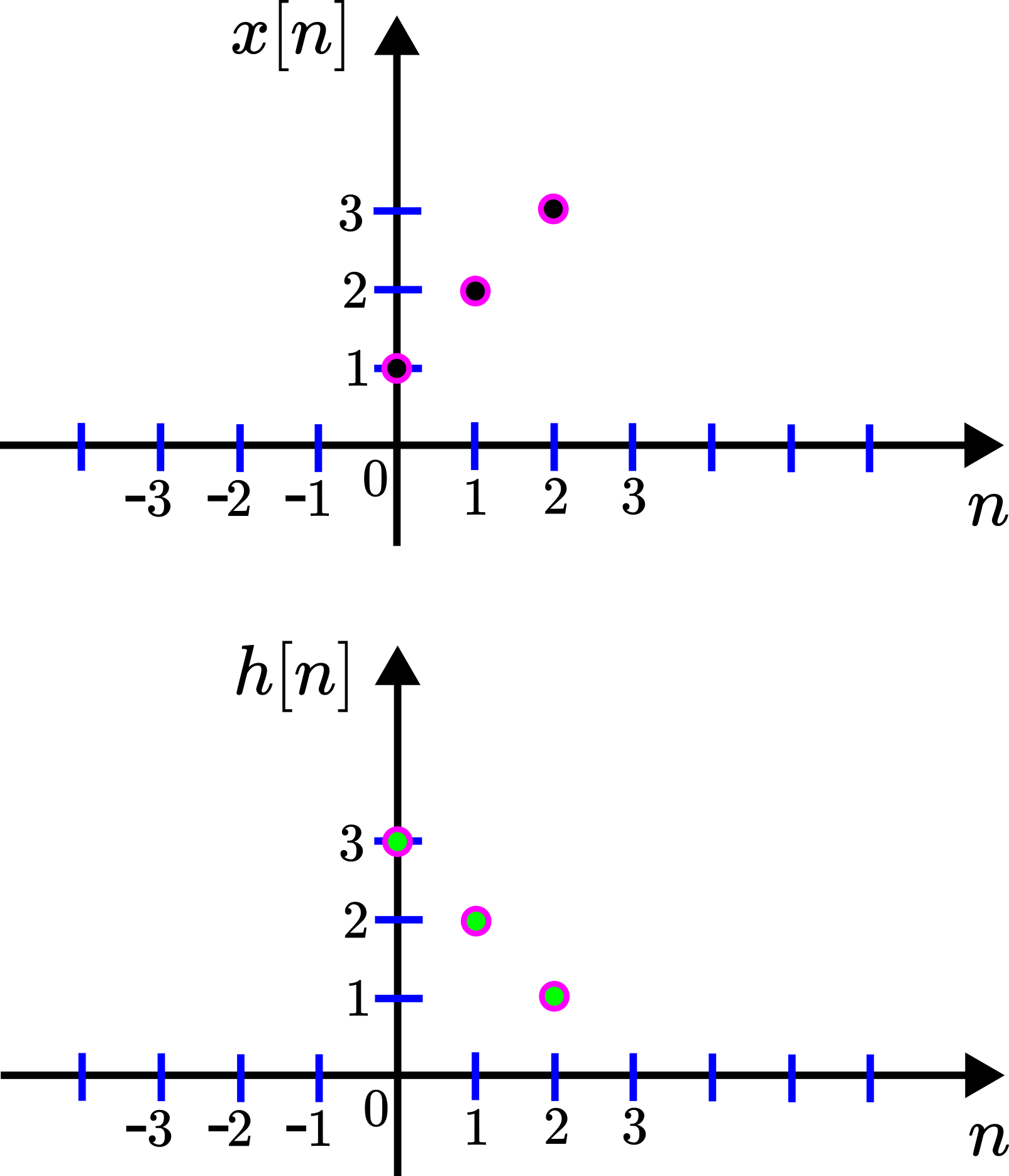
Example demonstrating convolution: Let the signals and be defined as follows
(5) ![\begin{align*}h[n] = \left\{ \begin{array}{ll} 3 & , \;\; n=0 \\ 2 &, \;\; n=1 \\ 1 &, \;\; n=2 \\ 0 &, \;\; \text{for all other integer} \;\; n \end{array} \right.\end{align*}](https://aleksandarhaber.com/wp-content/ql-cache/quicklatex.com-52eee092b35d3af5ceb9f2982d6a225a_l3.png "Rendered by QuickLaTeX.com")
(6) ![\begin{align*}x[n] = \left\{ \begin{array}{ll} 1 & , \;\; n=0 \\ 2 &, \;\; n=1 \\ 3 &, \;\; n=2 \\ 0 &, \;\; \text{for all other integer} \;\; n \end{array} \right.\end{align*}](https://aleksandarhaber.com/wp-content/ql-cache/quicklatex.com-f8d4c59a485fef60d9d0dce666941a4f_l3.png "Rendered by QuickLaTeX.com")
Compute the convolution sum
(7) ![\begin{align*}y[n]=\sum_{k=-\infty}^{+\infty}x[k]h[n-k]\end{align*}](https://aleksandarhaber.com/wp-content/ql-cache/quicklatex.com-6c17311dba44155fc1bbe758acd3f925_l3.png "Rendered by QuickLaTeX.com")
and give a graphical interpretation and derive a graphical method for computing the convolution sum.
Solution:
The figure below shows a graphical representation of two signals
First, taking into account that ![x[n]=0](https://aleksandarhaber.com/wp-content/ql-cache/quicklatex.com-3e6de1bdf5eac30a53b1953c753d01c3_l3.png "Rendered by QuickLaTeX.com") for negative values of , the sum (7) takes the following form
for negative values of , the sum (7) takes the following form
(8) ![\begin{align*}y[n] & =\sum_{k=0}^{+\infty}x[k]h[n-k] \\y[n] & =x[0]h[n]+x[1]h[n-1]+x[2]h[n-2]+x[3]h[n-3]+\ldots \end{align*}](https://aleksandarhaber.com/wp-content/ql-cache/quicklatex.com-54f0dcc744efd7134f874c1357461b16_l3.png "Rendered by QuickLaTeX.com")
Now, taking into account that ![x[n]\ne 0](https://aleksandarhaber.com/wp-content/ql-cache/quicklatex.com-06a213702b6b75950131c0f5467a2bc6_l3.png "Rendered by QuickLaTeX.com") only for
only for  , the convolution sum (8) takes the following form
(9) ![\begin{align*}y[n]=x[0]h[n]+x[1]h[n-1]+x[2]h[n-2]\end{align*}](https://aleksandarhaber.com/wp-content/ql-cache/quicklatex.com-61dd0486f2bb0f8471683a5cdfd7d42c_l3.png "Rendered by QuickLaTeX.com")
Let us now represent this sum for different values of . For  , we have
(10) ![\begin{align*}y[0] &=x[0]h[0]+x[1]h[-1]+x[2]h[-2] \\& = x[0]h[0]+x[1]0+x[2]0 \\& =x[0]h[0] =1\cdot 3=3\end{align*}](https://aleksandarhaber.com/wp-content/ql-cache/quicklatex.com-6a4864e320a0fc4cba27d8d6d3926882_l3.png "Rendered by QuickLaTeX.com")
For  , we have
(11) ![\begin{align*}y[1]& =x[0]h[1]+x[1]h[0]+x[2]h[-1] \\& =x[0]h[1]+x[1]h[0]+x[2]0 \\& =x[0]h[1]+x[1]h[0] =1\cdot 2 +2\cdot 3 = 8 \end{align*}](https://aleksandarhaber.com/wp-content/ql-cache/quicklatex.com-60f797d8681983e54703148b6a49651c_l3.png "Rendered by QuickLaTeX.com")
For  , we have
(12) ![\begin{align*}y[2]& =x[0]h[2]+x[1]h[1]+x[2]h[0]\\& =1 \cdot 1 +2 \cdot 2+3 \cdot 3 = 14\end{align*}](https://aleksandarhaber.com/wp-content/ql-cache/quicklatex.com-7fd078613b816921cc83cde171e7cfb6_l3.png "Rendered by QuickLaTeX.com")
For  , we have
(13) ![\begin{align*}y[3]& =x[0]h[3]+x[1]h[2]+x[2]h[1]\\& =x[0]\cdot 0 +x[1]h[2]+x[2]h[1] \\& = x[1]h[2]+x[2]h[1] =2 \cdot 1+ 3 \cdot 2 = 8 \end{align*}](https://aleksandarhaber.com/wp-content/ql-cache/quicklatex.com-a60d2a1db27aa0ab0bf8e36502190f0a_l3.png "Rendered by QuickLaTeX.com")
For  , we have
(14) ![\begin{align*}y[4] & =x[0]h[4]+x[1]h[3]+x[2]h[2] \\& =x[0]\cdot 0+x[1]\cdot 0+x[2]h[2] \\& = x[2]h[2] =3\cdot 1 = 3\end{align*}](https://aleksandarhaber.com/wp-content/ql-cache/quicklatex.com-d5a11ca35357af710bb272a7d4d97d70_l3.png "Rendered by QuickLaTeX.com")
To give a graphical interpretation of the convolution sum, let us analyze again the derived equations
(15) ![\begin{align*}& n=0,\;\; y[0]=x[0]h[0]+x[1]h[-1]+x[2]h[-2] \\& n=1,\;\; y[1]=x[0]h[1]+x[1]h[0]+x[2]h[-1] \\& n=2,\;\; y[2]=x[0]h[2]+x[1]h[1]+x[2]h[0] \\& n=3,\;\; y[3]=x[0]h[3]+x[1]h[2]+x[2]h[1] \\& n=4,\;\; y[4]=x[0]h[4]+x[1]h[3]+x[2]h[2]\end{align*}](https://aleksandarhaber.com/wp-content/ql-cache/quicklatex.com-9f02c0615c3baef30ebc63f54d2fa03a_l3.png "Rendered by QuickLaTeX.com")
We can observe the following
- In the sum terms, the position of the sequence stays the same as is increased.
- In the sum terms, the sequence is shifted in time at corresponding positions in the sum.
This means that in the graphical interpretation of the convolution sum, the sequence is fixed, and the sequence is shifted. However, the sequence has to be reversed or reflected with respect to the vertical axis. This is explained in the sequel. For that purpose, and for clarity, let us again write the general formula (9) as follows
(16) ![\begin{align*}y[n]=x[0]h[n]+x[1]h[n-1]+x[2]h[n-2]=\sum_{k=0}^{2}x[k]h[n-k]\end{align*}](https://aleksandarhaber.com/wp-content/ql-cache/quicklatex.com-3b3abf9dcb2ccf56870157bf58e996f1_l3.png "Rendered by QuickLaTeX.com")
From this formula, we have
(17) ![\begin{align*}& n=0,\;\; y[0]=x[0]h[0-0]+x[1]h[0-1]+x[2]h[0-2]=\sum_{k=0}^{2}x[k]h[0-k] \\& n=1,\;\; y[1]=x[0]h[1-0]+x[1]h[1-1]+x[2]h[1-2]=\sum_{k=0}^{2}x[k]h[1-k] \\& n=2,\;\; y[2]=x[0]h[2-0]+x[1]h[2-1]+x[2]h[2-2]=\sum_{k=0}^{2}x[k]h[2-k] \\& n=3,\;\; y[3]=x[0]h[3-0]+x[1]h[3-1]+x[2]h[3-2]=\sum_{k=0}^{2}x[k]h[3-k] \\& n=4,\;\; y[4]=x[0]h[4-0]+x[1]h[4-1]+x[2]h[4-2]=\sum_{k=0}^{2}x[k]h[4-k]\end{align*}](https://aleksandarhaber.com/wp-content/ql-cache/quicklatex.com-aeba5bdbfbfef8475d4f0282074858b5_l3.png "Rendered by QuickLaTeX.com")
In these sums, we can think of the sequence ![h[n-k]](https://aleksandarhaber.com/wp-content/ql-cache/quicklatex.com-e9c5ba1666ca08fb731e6c9da4d336e7_l3.png "Rendered by QuickLaTeX.com") ,
,  , as the sequence
 ![h[-k]](https://aleksandarhaber.com/wp-content/ql-cache/quicklatex.com-028d8cbe0e5a5bace50c828be29c8da0_l3.png "Rendered by QuickLaTeX.com") that is shifted (delayed) for time steps.
that is shifted (delayed) for time steps.
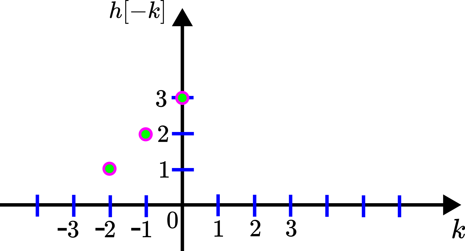
Let us further elaborate on how the sequence is constructed from the sequence ![h[k]](https://aleksandarhaber.com/wp-content/ql-cache/quicklatex.com-3d5b8a041a243c7ba0db4ee2ff3740e9_l3.png "Rendered by QuickLaTeX.com") or . Let us denote the sequence by
or . Let us denote the sequence by ![h_{1}[k]](https://aleksandarhaber.com/wp-content/ql-cache/quicklatex.com-0d19b6334871698289ed592d4d87e696_l3.png "Rendered by QuickLaTeX.com") . That is,
. That is,
(18) ![\begin{align*}h_{1}[k]=h[-k]\end{align*}](https://aleksandarhaber.com/wp-content/ql-cache/quicklatex.com-9fd34e301b7c0998eec58615667e859f_l3.png "Rendered by QuickLaTeX.com")
Taking into account the definition of the sequence , for  , the sequence is
(19) ![\begin{align*}k=0,\; => \; h_{1}[0]=h[0]=3 \\k=-1,\; => \;h_{1}[-1]= h[-(-1)]=h[1]=2 \\k=-2,\; => \; h_{1}[-2]= h[-(-2)]=h[2]=1 \\\text{for all other values of} \;\; k \;\; =>\; h_{1}[k]=h[-k]=0\end{align*}](https://aleksandarhaber.com/wp-content/ql-cache/quicklatex.com-a26bcf2ef00d50ade7373287b2224e2e_l3.png "Rendered by QuickLaTeX.com")
This is actually the original sequence that is mirrored or reflected with respect to the vertical axis . This sequence is illustrated in the figure below.
 .
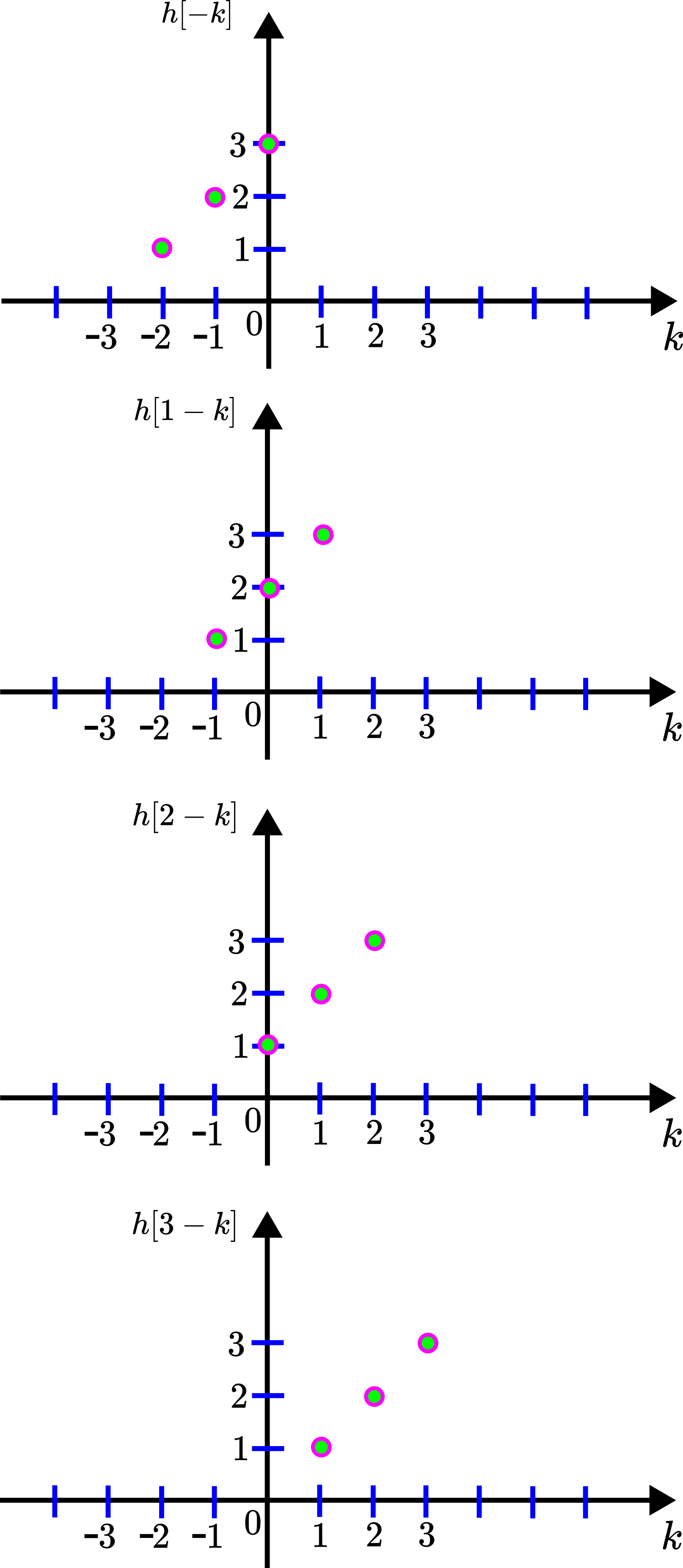
.If we delay or shift this sequence in time, we will obtain the following sequences for different values of the time delay:
 delayed for
  ,
,  ,
,  , and
, and  time steps.
These shifted or delayed sequences constructed on the basis of , will help us to graphically interpret the convolution sum.
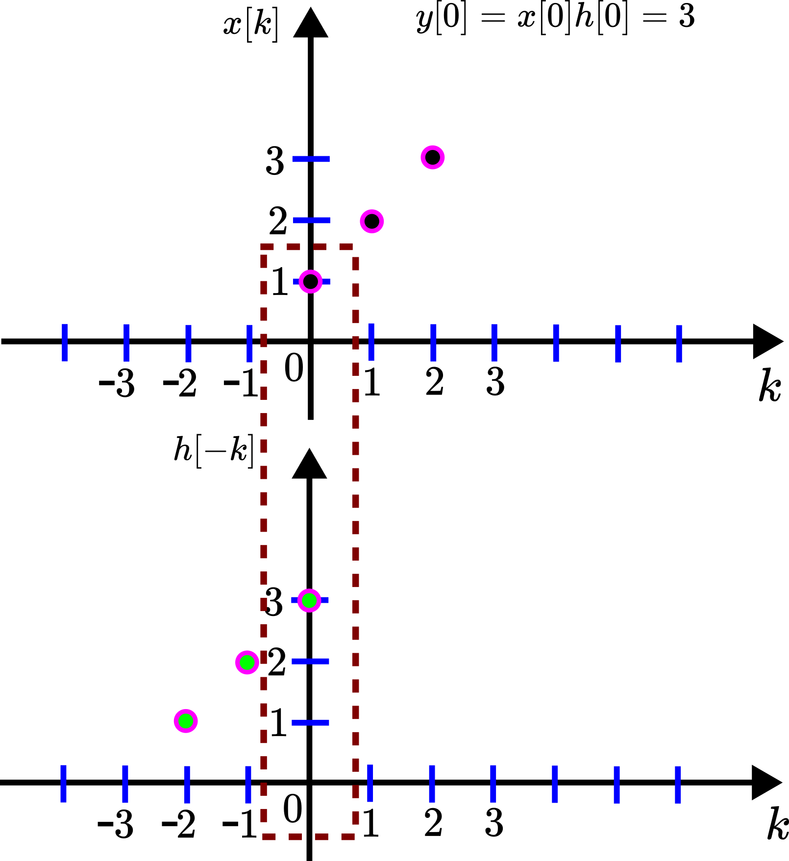
Let us start with
(20) ![\begin{align*}n=0,\;\; y[0]=x[0]h[0-0]+x[1]h[0-1]+x[2]h[0-2] =x[0]h[0]\end{align*}](https://aleksandarhaber.com/wp-content/ql-cache/quicklatex.com-1c2c26db1fdf11b6428497df28697d45_l3.png "Rendered by QuickLaTeX.com")
This sum has the graphical interpretation given in the figure below.
![y[0]](https://aleksandarhaber.com/wp-content/ql-cache/quicklatex.com-303eaebff2cb2159ebc878229caa4eed_l3.png "Rendered by QuickLaTeX.com") .
.We only multiply the terms of the sequences ![x[k]](https://aleksandarhaber.com/wp-content/ql-cache/quicklatex.com-88be78b31528bb450106ef8a8ee13b12_l3.png "Rendered by QuickLaTeX.com") and that are in the dashed rectangle.
and that are in the dashed rectangle.
For , we have
(21) ![\begin{align*} n=1,\;\; y[1]=x[0]h[1-0]+x[1]h[1-1]+x[2]h[1-2]= x[0]h[1]+x[1]h[0] \end{align*}](https://aleksandarhaber.com/wp-content/ql-cache/quicklatex.com-950f3a1288eb3273778643526dff8b14_l3.png "Rendered by QuickLaTeX.com")
This sum has the graphical interpretation given in the figure below.
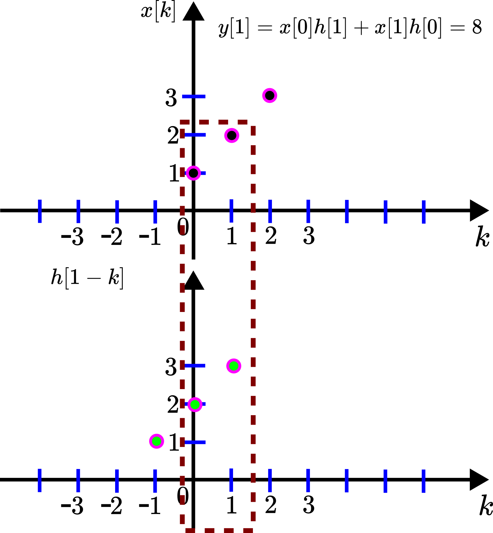
![y[1]](https://aleksandarhaber.com/wp-content/ql-cache/quicklatex.com-5c130d8a2453ab754d4f44b240ec527e_l3.png "Rendered by QuickLaTeX.com") .
.We delay the sequence to obtain ![h[1-k]](https://aleksandarhaber.com/wp-content/ql-cache/quicklatex.com-5b788500dcda6fde821567c81215f0d6_l3.png "Rendered by QuickLaTeX.com") , and we only multiply the terms of the sequences and that are in the dashed rectangle.
, and we only multiply the terms of the sequences and that are in the dashed rectangle.
For , we have
(22) ![\begin{align*} n=2,\;\; y[2]=x[0]h[2-0]+x[1]h[2-1]+x[2]h[2-2]=x[0]h[2]+x[1]h[1]+x[2]h[0]\end{align*}](https://aleksandarhaber.com/wp-content/ql-cache/quicklatex.com-e5586322ee8b5b5c92fa536fed045071_l3.png "Rendered by QuickLaTeX.com")
This sum has the graphical interpretation given in the figure below.
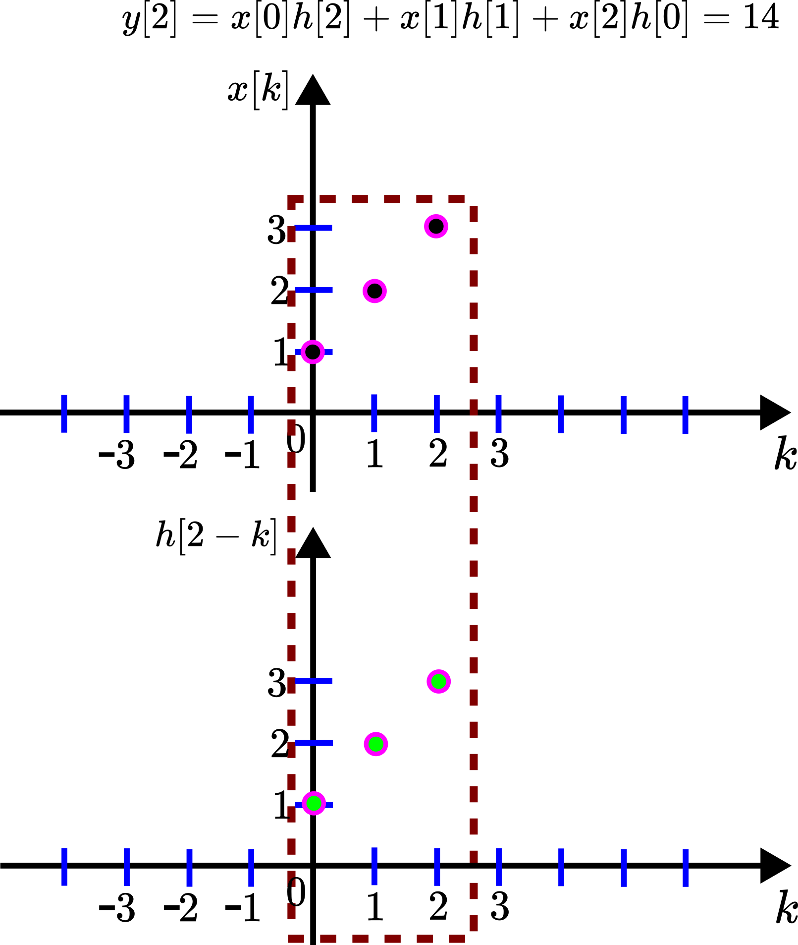
![y[2]](https://aleksandarhaber.com/wp-content/ql-cache/quicklatex.com-80430bda773bf7cb6ca603292b7c979c_l3.png "Rendered by QuickLaTeX.com") .
.We delay the sequence to obtain ![h[2-k]](https://aleksandarhaber.com/wp-content/ql-cache/quicklatex.com-f543fd5cc3d30321de8c8317b40a9c0d_l3.png "Rendered by QuickLaTeX.com") , and we only multiply the terms of the sequences and that are in the dashed rectangle.
, and we only multiply the terms of the sequences and that are in the dashed rectangle.
For , we have
(23) ![\begin{align*} n=3,\;\; y[3]=x[0]h[3-0]+x[1]h[3-1]+x[2]h[3-2]=x[1]h[2]+x[2]h[1]\end{align*}](https://aleksandarhaber.com/wp-content/ql-cache/quicklatex.com-63db74caa555745c39905ebcd4e643df_l3.png "Rendered by QuickLaTeX.com")
This sum has the graphical interpretation given in the figure below.
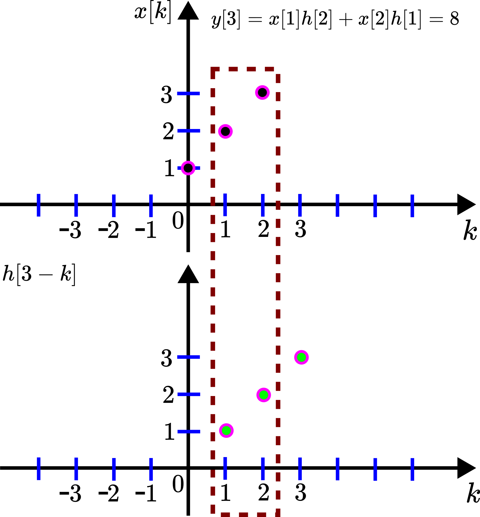
![y[3]](https://aleksandarhaber.com/wp-content/ql-cache/quicklatex.com-0fa142f298bea8e6a16d4376658755a1_l3.png "Rendered by QuickLaTeX.com") .
.We delay the sequence to obtain ![h[3-k]](https://aleksandarhaber.com/wp-content/ql-cache/quicklatex.com-5663eb646a01514b8a674a8f4ff30e54_l3.png "Rendered by QuickLaTeX.com") , and we only multiply the terms of the sequences and that are in the dashed rectangle.
, and we only multiply the terms of the sequences and that are in the dashed rectangle.
For , we have
(24) ![\begin{align*} n=4,\;\; y[4]=x[0]h[4-0]+x[1]h[4-1]+x[2]h[4-2]=x[2]h[2]\end{align*}](https://aleksandarhaber.com/wp-content/ql-cache/quicklatex.com-aed104e7f8bd335a837e6837b6858e24_l3.png "Rendered by QuickLaTeX.com")
This sum has the graphical interpretation given in the figure below.
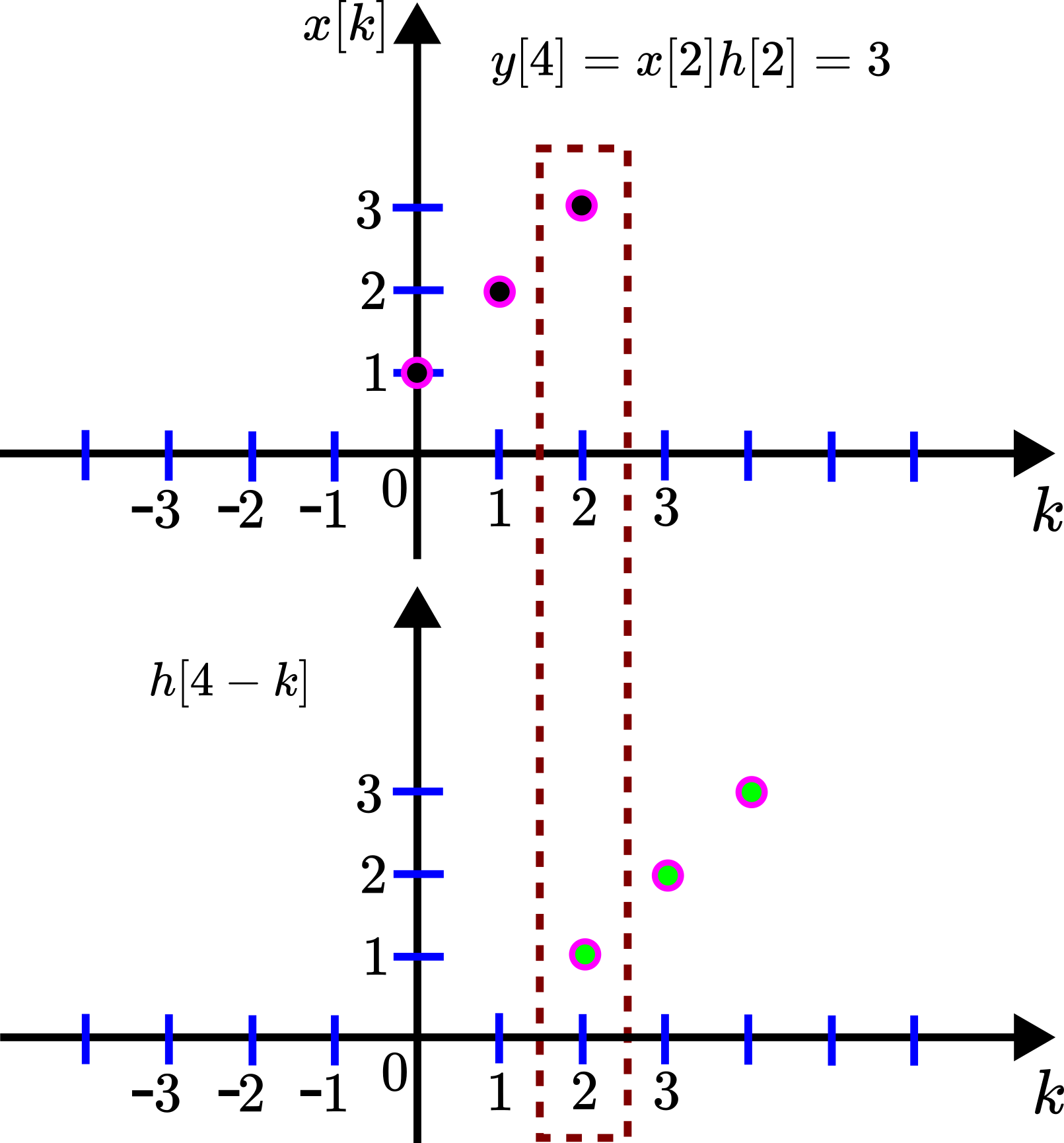
![y[4]](https://aleksandarhaber.com/wp-content/ql-cache/quicklatex.com-58cd652f501eca4f303f36c7dbcec9c3_l3.png "Rendered by QuickLaTeX.com") .
.We delay the sequence to obtain ![h[4-k]](https://aleksandarhaber.com/wp-content/ql-cache/quicklatex.com-5fb51b1025ee6ca83a4a61901ecab593_l3.png "Rendered by QuickLaTeX.com") , and we only multiply the terms of the sequences and that are in the dashed rectangle.
, and we only multiply the terms of the sequences and that are in the dashed rectangle.
Convolution in MATLAB
The following MATLAB script will compute convolution
x = [1 2 3];
h = [3 2 1];
y = conv(x,h,'full')
The output is
y =

     3     8    14     8     3
We used the MATLAB function conv() to compute the convolution. The MATLAB script is self-explanatory.