Numerical Solution of Forward Kinematics Problem of Differential Drive Robot and 2D Simulation/Animation of Trajectory in Python and Pygame – Fusion of Engineering, Control, Coding, Machine Learning, and Science

In this robotics and mechatronics tutorial, we explain how to numerically solve the forward kinematics problem of a differential drive robot (differential wheeled robot). Furthermore, we explain how to simulate and animate the computed robot trajectories by using Python and Pygame. Pygame is an open-source and free game development environment in Python. It can be used to simulate and animate the trajectories of mobile robots. This tutorial is very important for students, engineers, and professors who want to visualize robot motion, path planning, and SLAM algorithms. The advantages of the methods that we are presenting are that they are very simple and open source. Consequently, you can completely understand and track every aspect of simulation and animation. In this tutorial, you will learn

How to formulate the forward kinematics problem for mobile robots.
How to numerically solve forward kinematics problems in Python.
How to visualize the mobile robot motion in Python and Pygame and how to generate amazing simulations.

The YouTube tutorial accompanying this webpage tutorial is given below.

Forward Kinematics of Differential Drive Robot – Problem Statement

In our previous tutorial, whose link is given here, we derived the kinematics equations of the differential drive robot. Here, for completeness of this tutorial, we will briefly summarize the robot description and kinematics equations. The robot kinematic diagram is shown in the figure below.

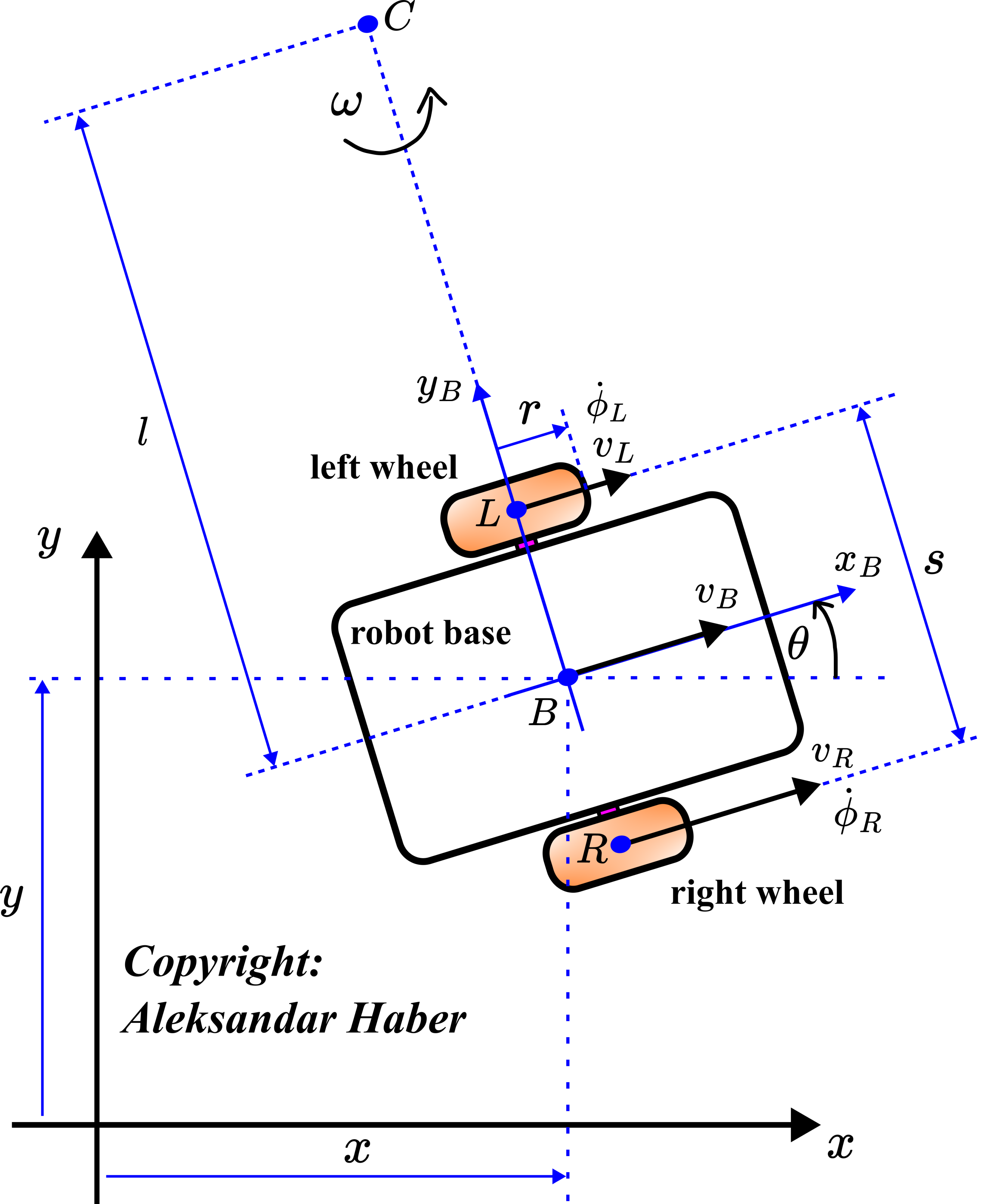
Figure 1: Kinematics diagram of the differential drive robot.

The symbols used in this figure are explained below.

$x$ and $y$ are the translation coordinates of the body frame attached to the point $B$ with respect to the inertial frame $x-y$ .
$\theta$ is the angle of rotation of the robot which is at the same time the angle between the body frame and the inertial frame.
$x_{B}$ and $y_{B}$ are the coordinates in the body frame and at the same time they denote the axes of the body frame.
$C$ is the instantaneous center of rotation.
$\omega$ is the instantaneous angular velocity of the robot body.
$L$ is the center point of the left wheel.
$R$ is the center point of the right wheel.
$B$ is the middle point between the points $L$ and $R$ .
$v_{L}$ is the velocity of the center of the left wheel.
$v_{R}$ is the velocity of the center of the right wheel.
$v_{B}$ is the velocity of the point $B$ .
$\dot{\phi}_{L}$ is the angular velocity of the left wheel.
$\dot{\phi}_{R}$ is the angular velocity of the right wheel.
$l$ is the distance between the point $B$ and the point $C$ .
$r$ is the radius of the wheels.
$s$ is the distance between the points $L$ and $R$ .
$\dot{x}$ is the projection of the velocity $v_{B}$ on the $x$ axis.
$\dot{y}$ is the projection of the velocity $v_{B}$ on the $y$ axis.

The kinematics equations can take two forms. The first form is expressed by using the velocities of the right and left wheels is given below.

(1) $\begin{align*}\dot{x}& =\frac{v_{L}}{2}\cos(\theta)+\frac{v_{R}}{2}\cos(\theta) \\\dot{y}& =\frac{v_{L}}{2}\sin(\theta)+\frac{v_{R}}{2}\sin(\theta) \\\dot{\theta} & = -\frac{1}{s}v_{L}+ \frac{1}{s}v_{R}\end{align*}$

Taking into account that $v_{L}=r\dot{\phi}_{L}$ and $v_{R}=r\dot{\phi}_{R}$ , we can expressed the system of last equations as follows

(2) $\begin{align*}\dot{x}& =\frac{r\dot{\phi}_{L}}{2}\cos(\theta) +\frac{r\dot{\phi}_{R}}{2}\cos(\theta) \\\dot{y}& =\frac{r\dot{\phi}_{L}}{2}\sin(\theta) +\frac{r\dot{\phi}_{R}}{2}\sin(\theta) \\\dot{\theta} & = -\frac{r}{s}\dot{\phi}_{L}+ \frac{r}{s}\dot{\phi}_{R}\end{align*}$

In our simulations, we will use the second form of kinematics equations given by the system of equations (2).

Classical Forward Kinematics Problem Formulation: Let us assume that the left and right wheel rotation angles $\phi_{L}$ and $\phi_{R}$ as given as functions of time. That is, we assume that $\phi_{L}=\phi_{L}(t)$ and $\phi_{R}=\phi_{R}(t)$ are given. Then, the forward kinematics problem is to determine $x$ , $y$ , and $\theta$ as functions of time. That is, we want to determine functions that describe the $x$ and $y$ positions of the robot point $B$ and the angle rotation of the robot body $\theta$ as functions of time.

If we know $\phi_{L}=\phi_{L}(t)$ and $\phi_{R}=\phi_{R}(t)$ as functions of time, then we can differentiate these quantities with respect to time to determine the angular velocities $\dot{\phi}_{L}=\dot{\phi}_{L}(t)$ and $\dot{\phi}_{R}=\dot{\phi}_{R}(t)$ as functions of time. Then, we can formulate the forward kinematics problem in terms of angular velocities.

Forward Kinematics Problem Formulation by Using Angular Velocities: Let us assume that the left and right wheel angular velocities $\dot{\phi}_{L}$ and $\dot{\phi}_{R}$ as given as functions of time. That is, we assume that $\dot{\phi}_{L}=\dot{\phi}_{L}(t)$ and $\dot{\phi}_{R}=\dot{\phi}_{R}(t)$ are given. Then, the forward kinematics problem is to determine $x$ , $y$ , and $\theta$ as functions of time. That is, we want to determine functions that describe the $x$ and $y$ positions of the robot point $B$ and the angle rotation of the robot body $\theta$ as functions of time.

Before we continue with explanations, we have to explain the general philosophy of forward kinematics problems. Forward kinematics problems are also known as direct kinematics problems. In general terms, the problem is to transform the local coordinate description into the global coordinate description. For example, in the case of robot manipulators, the forward kinematics problem is to calculate the position of the center point of the end effector in the global Cartesian coordinate system, by using the information about rotation angles of robot joints and robot geometric and kinematic parameters. That is, we search for local to global transformation. In the case of the mobile robot, the local coordinates are wheel rotation angles, since wheels play the role of joints. The global coordinates are the position of the robot $x$ and $y$ with respect to the inertial frame and the orientation of the robot body $\theta$ .

Numerical Solution of Forward Kinematics Problem in Python

For simplicity, we solve the forward kinematics problem formulation by using angular velocities. Obviously, to solve the forward kinematics problem, we need to integrate the system of equations (2). Under certain conditions and assumptions, we can “exactly” solve this differential system of equations by evaluating integrals. However, in the general case, this might not be possible. Consequently, we use numerical integration methods to solve the forward kinematics problem.

To solve the problem, we use the Python function odeint(). The code is given below.

# -*- coding: utf-8 -*-
"""
Differential Drive Mobile Robot Simulation in Pygame
- This file solves the forward (direct)
kinematics problem
Author: Aleksandar Haber 
Date: October 2023
"""

import numpy as np
from scipy.integrate import odeint
import matplotlib.pyplot as plt

# define the robot parameters
# wheel radius 
r=15
# distance between the wheel centers
s=4*r

# time vector
timeVector=np.linspace(0,100,10000)

# here you define the robot control variables
# left wheel angular velocity
dphiLA=2*np.ones(timeVector.shape)
# right wheel angular velocity
dphiRA=1.4*np.ones(timeVector.shape)

# this function defines a system of differential equations 
# defining the forward kinematics 
# x[0]=x, x[1]=y, x[2]=theta
def diffModel(x,t,timePoints,sC,rC,dphiLArray,dphiRarray):
    #value of dphiL at the current time t 
    dphiLt=np.interp(t,timePoints, dphiLArray)
    #value of dphiR at the current time t 
    dphiRt=np.interp(t,timePoints, dphiRarray)
    
    # \dot{x}
    dxdt=0.5*rC*dphiLt*np.cos(x[2])+0.5*rC*dphiRt*np.cos(x[2])
    # \dot{x}
    dydt=0.5*rC*dphiLt*np.sin(x[2])+0.5*rC*dphiRt*np.sin(x[2])
    # \dot{\theta}
    dthetadt=-(rC/sC)*dphiLt+(rC/sC)*dphiRt
    
    # right-side of the state equation
    dxdt=[dxdt,dydt,dthetadt]
    return dxdt
    


# define the initial values for simulation 
# x,y,theta
initialState=np.array([500,500,0])
# solve the forward kinematics problem
solutionArray=odeint(diffModel,initialState,timeVector,
                     args=(timeVector,s,r,dphiLA,dphiRA))

# save the simulation data
np.save('simulationData.npy', solutionArray)

# plot the results 
plt.plot(timeVector, solutionArray[:,0],'b',label='x')
plt.plot(timeVector, solutionArray[:,1],'r',label='y')
plt.plot(timeVector, solutionArray[:,2],'m',label='theta')
plt.xlabel('time')
plt.ylabel('x,y,theta')
plt.legend()
plt.savefig('simulationResult.png',dpi=600)
plt.show()

First, we define the robot parameters $s$ and $r$ . Then we define the simulation time vector “timeVector”. Then, we define the left and right wheel velocities. The velocities are defined as vectors “dphiLA” (left) and “dphiRA” (right), where every entry of the vector is the velocity at the corresponding time instant. That is, we define velocity functions in the discrete-time domain. We assume that the velocities are constant. This means that the robot point $B$ will describe a circular trajectory. For a detailed explanation of why the robot will describe the circular trajectory in this case, see our previous tutorial given here.

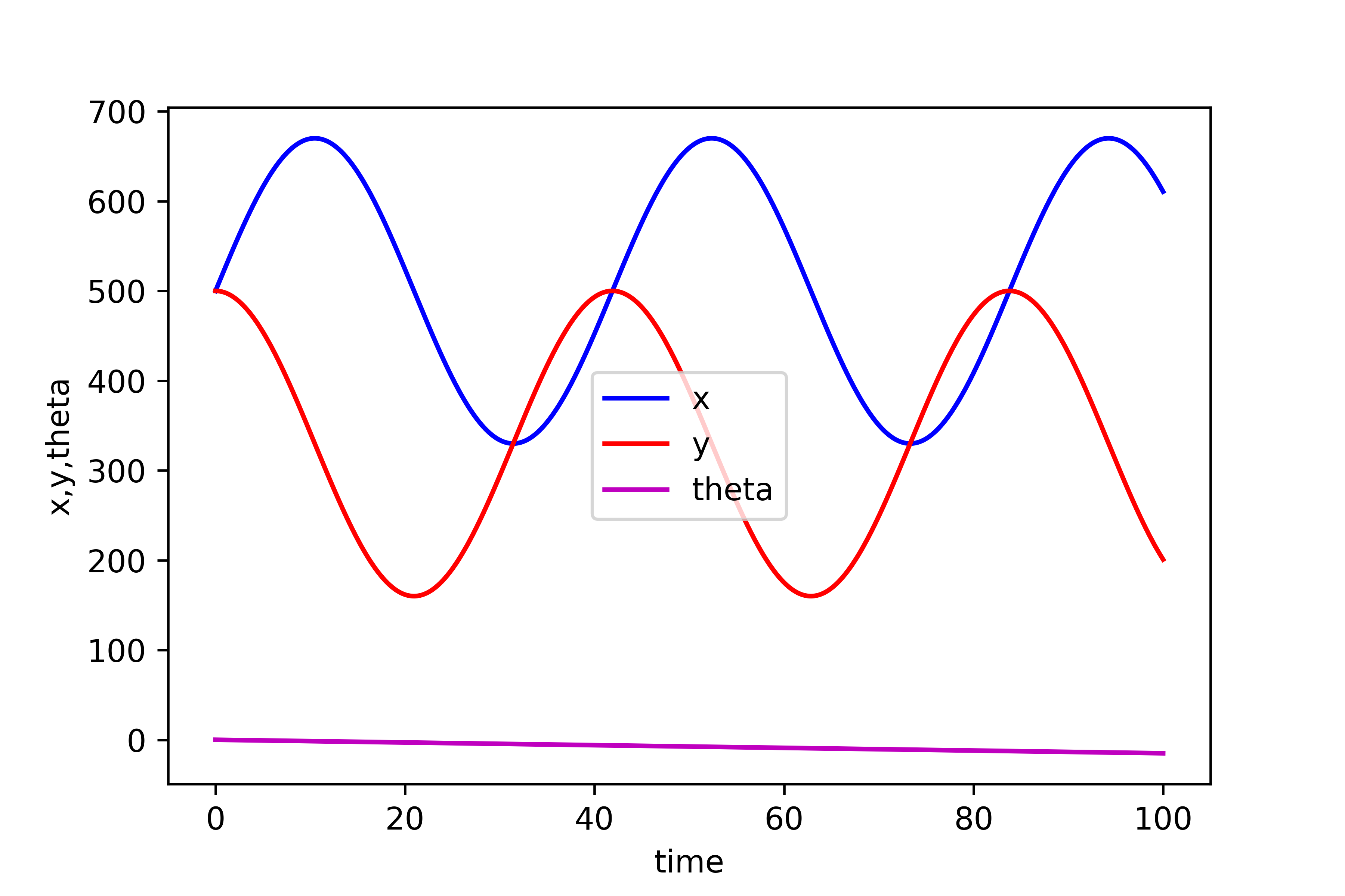
Then, the function “diffModel” defines the kinematics differential equations (2). For a given value of the vector $\mathbf{x}$ , this function will return the right-hand side of the equation (2). The entries of the vector $\mathbf{x}$ are $x$ , $y$ , and $\theta$ coordinates. Then, we define the initial values of the positions and angles for simulations. Finally, we use the function “odeint()” to integrate the kinematics equations. We save the data in files such that we can use them in Pygame scripts, and plot the results. The trajectories are given in the figure below.

Next, we visualize the results by using the Pygame script given below.

# -*- coding: utf-8 -*-
"""
Differential Drive Mobile Robot Simulation in Pygame
- This code creates robot animation on the basis of the 
simulation data obtained by solving the forward (direct)
kinematics problem
Author: Aleksandar Haber 
Date: October 2023
"""

# pip install pygame
import pygame
import numpy as np
 
# Initialise pygame
pygame.init()
 
# Set window size
size = width,height = 1200, 800
screen = pygame.display.set_mode(size)
# Clock
clock = pygame.time.Clock()
# Load robot image
image = pygame.image.load('robot_model2.png').convert_alpha()

# we need to adjust the robot image size
robot_image_size = (150, 150)
# Scale the image to your needed size
image = pygame.transform.scale(image, robot_image_size)
 

# this is a frame counter
i=0
# load the simulation data that is computed by solving the direct kinematics 
# problem
solutionArray = np.load('simulationData.npy')

# x coordinate of the center of the robot
x=solutionArray[:,0]
# y coordinate of the center of the robot
y=solutionArray[:,1]
# rotation angle, has to be converted from radians to degrees 
# also, we have to multiply with -1 since the vertical axis in animation 
# is reversed
angle=-1*(360/(2*np.pi))*solutionArray[:,2]


# this list is used to store tuples of coordinates for tracking and ploting 
# the robot trajectory
coordinates=[]
# trajectory color 
color_trajectory = ( 255,255,153 )
while (i<len(x)):
     # Close window event
    for event in pygame.event.get():
        if event.type == pygame.QUIT:
            running = True
         
    # Background Color
    screen.fill((0, 0, 0))
    
    # over here we rotate an image and create a copy of the rotated image 
    image1 = pygame.transform.rotate(image,angle[i])
    # then we return a rectangle corresponding to the rotated copy
    # the rectangle center is specified as an argument
    image1_rect = image1.get_rect(center=(x[i], y[i]))
    # then we plot the rotated image copy with boundaries specified by 
    # the rectangle
    screen.blit(image1, image1_rect)
    # here, we append the trajectory, such that we can plot it    
    coordinates.append((x[i],y[i]))
    # plot the line only if we have more than 1 point 
    if i>1:
        pygame.draw.lines( screen, color_trajectory, False, coordinates,6 ) 
   
    # Part of event loop
    pygame.display.flip()
    # introduce a delay
    pygame.time.delay(1)
    # https://www.pygame.org/docs/ref/time.html#pygame.time.Clock.tick
    clock.tick(100)
    i=i+1

# this is important, run this if the pygame window does not want to close
pygame.quit()

This script is explained in our next tutorial, whose link is given over here. Briefly speaking, this code will load the data generated by the script for solving the forward kinematics problem and it will generate the robot animation. The robot animation is given below.

Forward Kinematics of Differential Drive Robot – Problem Statement

Numerical Solution of Forward Kinematics Problem in Python

admin

You might also like

Dynamical Model of a Tank (Reservoir) Filled with Liquid and Simulation in Python

How to install Python in VS Code and How to Debug and Install Packages in Virtual Environment

Quadratic Forms, Positive Definite, Negative Definite, and Semi-Definite Matrices