Disciplined Kalman Filter Implementation in Python by Using Object-Oriented Approach – Fusion of Engineering, Control, Coding, Machine Learning, and Science

In our previous post, which can be found here, we explained how to derive the Kalman filter equations from scratch by using the recursive least squares method. In this post, we explain how to implement the Kalman filter in Python. For implementing the Kalman filter we will use an objected-oriented approach with the goal of creating a reusable and easy-to-understand code. The Python codes accompanying this tutorial are given here. The YouTube video accompanying this post is given below.

Summary of the Kalman Filter Equations

The Kalman filter equations that are derived in our previous tutorial, have the following form:

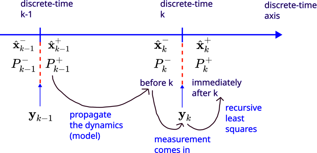
Step 1: Propagate the a posteriori estimate $\hat{\mathbf{x}}_{k-1}^{+}$ and the covariance matrix of the estimation error $P_{k-1}^{+}$ , through the system dynamics to obtain the a priori state estimate and the covariance matrix of the estimation error for the step $k$ :

(1) $\begin{align*}\hat{\mathbf{x}}_{k}^{-}& =A_{k-1}\mathbf{x}_{k-1}^{+}+B_{k-1}\mathbf{u}_{k-1} \\P_{k}^{-}& =A_{k-1}P_{k-1}^{+}A_{k-1}^{T}+Q_{k-1}\end{align*}$

Step 2: Obtain the measurement $\mathbf{y}_{k}$ . Use this measurement, and the a priori estimate $\hat{\mathbf{x}}_{k}^{-}$ and the covariance matrix of the estimation error $P_{k}^{-}$ to compute the a posteriori state estimate and the covariance matrix of the estimation error

(2) $\begin{align*}K_{k} & =P_{k}^{-}C_{k}^{T}(R_{k}+C_{k}P_{k}^{-}C_{k}^{T})^{-1} \\\hat{\mathbf{x}}_{k}^{+} & = \hat{\mathbf{x}}_{k}^{-}+K_{k}(\mathbf{y}_{k}-C_{k}\hat{\mathbf{x}}_{k}^{-}) \\P_{k}^{+}&=(I-K_{k}C_{k})P_{k}^{-}(I-K_{k}C_{k})^{T}+K_{k}R_{k}K_{k}^{T} \\P_{k}^{+}& =(I-K_{k}C_{k})P_{k}^{-} \end{align*}$

In these equations, $\hat{\mathbf{x}}_{k}^{-}$ is the a priori state estimate, $\hat{\mathbf{x}}_{k}^{+}$ is the a posterior state estimate, $k$ is the discrete-time instant, $A_{k-1},B_{k-1}$ and $C_{k-1}$ are the system matrices, $Q_{k-1}$ is the process noise covariance matrix, $R_{k-1}$ is the measurement noise covariance matrix, $I$ is an identity matrix, $P_{k}^{+}$ is the a posteriori covariance matrix of the estimation error, and $P_{k}^{+}$ is the a priori covariance matrix of the estimation error.

These steps are graphically illustrated in Fig. 1 below.

Figure 1: Graphical illustration of the Kalman filter steps.

Test Example

Here, we present a test example that will be used to check the implementation accuracy and performance. We consider a Newtonian particle moving with a constant acceleration $a$ :

(3) $\begin{align*}\ddot{x}=a\end{align*}$

where $a$ is the constant acceleration, and $x=x(t)$ is a position of the particle, $t$ is time, and $\ddot{x}$ is the second derivative of the position $x(t)$ . Physically, this system can be seen as a vehicle moving in a straight line with constant acceleration. By integrating the equation (3) twice, we obtain the position $x(t)$ :

(4) $\begin{align*}x(t)=x_{0}+w_{0}t+\frac{1}{2}at^{2}\end{align*}$

where $x_{0}$ is an initial position and $w_{0}$ is an initial velocity,

We assume that the acceleration is not known, as well as the initial position and initial velocity. We assume that only the position is measured. However, the position observations are corrupted by the measurement noise.

Our goal is to estimate the position $x$ , velocity $\dot{x}$ , and acceleration $\ddot{x}$ from the noisy observations of the position $x$ .

Our first goal is to write a state-space model corresponding to the system (3). We introduce the state-space variables

(5) $\begin{align*}x_{1}&=x\\x_{2}&=\dot{x} \\x_{3}&=\ddot{x}\end{align*}$

From (3) and (5), we have

(6) $\begin{align*}\dot{x}_{1}&=x_{2} \\\dot{x}_{2}&=x_{3} \\\dot{x}_{3}&=0, \;\;\;\; \text{since the acceleration is constant} \end{align*}$

From (15), we have

(7) $\begin{align*}\underbrace{\begin{bmatrix}\dot{x}_{1}\\ \dot{x}_{2} \\ \dot{x}_{3} \end{bmatrix}}_{\dot{\mathbf{x}}}=\underbrace{\begin{bmatrix} 0 & 1 & 0 \\ 0 & 0 & 1\\ 0 & 0 & 0 \end{bmatrix}}_{A_{c}}\underbrace{\begin{bmatrix}x_{1}\\ x_{2} \\ x_{3} \end{bmatrix}}_{\mathbf{x}}\end{align*}$

where $A_{c}$ is the continuous state-space matrix. The next step is to discretize the state-space model (15). It is very well-known fact in control theory, that for the time interval of length $h$ , we have

(8) $\begin{align*}\mathbf{x}(k\cdot h)=e^{A_{c} h} \mathbf{x}((k-1)\cdot h)\end{align*}$

By defining $\mathbf{x}(k\cdot h)=\mathbf{x}_{k}$ and $\mathbf{x}((k-1)\cdot h)=\mathbf{x}_{k-1}$ , from (8), we obtain

(9) $\begin{align*}\mathbf{x}_{k}=A \mathbf{x}_{k-1}\end{align*}$

where the matrix $A$ is defined

(10) $\begin{align*}A=e^{A_{c} h}\end{align*}$

The number $h$ is the discretization period or the sampling period. We need to compute the matrix exponential. For that purpose, we can use the series expansion

(11) $\begin{align*}A= e^{A_{c} h} = I + A_{c}h+\frac{(A_{c}h)^{2}}{2!}+\ldots\end{align*}$

Let us compute (11). We have

(12) $\begin{align*}A_{c}h=\begin{bmatrix} 0 & 1 & 0 \\ 0 & 0 & 1 \\ 0 & 0 & 0 \end{bmatrix}h=\begin{bmatrix} 0 & h & 0 \\ 0 & 0 & h \\ 0 & 0 & 0 \end{bmatrix}\end{align*}$

(13) $\begin{align*}\frac{(A_{c}h)^{2}}{2!}=\frac{h^2}{2}\begin{bmatrix} 0 & 1 & 0 \\ 0 & 0 & 1 \\ 0 & 0 & 0 \end{bmatrix}\begin{bmatrix} 0 & 1 & 0 \\ 0 & 0 & 1 \\ 0 & 0 & 0 \end{bmatrix}=\frac{h^2}{2} \begin{bmatrix} 0 & 0 & 1 \\ 0 & 0 & 0 \\ 0 & 0 & 0 \end{bmatrix} = \begin{bmatrix} 0 & 0 & \frac{h^2}{2} \\ 0 & 0 & 0 \\ 0 & 0 & 0 \end{bmatrix} \end{align*}$

The powers of $A$ larger than $3$ in (11) are zero. Consequently, they do not need to be computed. Taking this fact into account, and by substituting (12) and (13) in (11), we obtain

(14) $\begin{align*}A= e^{A_{c} h} = \begin{bmatrix}1 & h & \frac{h^2}{2} \\ 0 & 1 & h \\ 0 & 0 & 1 \end{bmatrix}\end{align*}$

Under the assumption that only the position $x_{1}=x(t)$ can be measured, our state-space model takes the following form

(15) $\begin{align*}\mathbf{x}_{k} & =A\mathbf{x}_{k-1} \\\mathbf{y}_{k} & =C\mathbf{x}_{k}+v_{k}\end{align*}$

where

(16) $\begin{align*}C=\begin{bmatrix} 1 & 0 & 0 \end{bmatrix}\end{align*}$

is the measurement matrix $C$ and $v_{k}$ is the scalar measurement noise, with the covariance matrix (in our case, the covariance matrix is a scalar variable)

(17) $\begin{align*}R=\sigma^{2}\end{align*}$

Here we assume that the process noise is zero. Consequently, the process noise covariance matrix $Q$ is a zero matrix.

Object-oriented Python Implementation of the Kalman Filter

The Python codes accompanying this tutorial are given here. In the sequel, we explain these code files. We define a class called KalmanFilter. This class initializes and stores the important matrices and variables. Also, this class contains two methods (functions) that are implementing the step 1 and step 2 of the Kalman filter. The class implementation is given below.

class KalmanFilter(object):
    
    # x0 - initial guess of the state vector 
    # P0 - initial guess of the covariance matrix of the state estimation error
    # A,B,C - system matrices describing the system model
    # Q - covariance matrix of the process noise 
    # R - covariance matrix of the measurement noise
    
    def __init__(self,x0,P0,A,B,C,Q,R):
        
        # initialize vectors and matrices
        self.x0=x0
        self.P0=P0
        self.A=A
        self.B=B
        self.C=C
        self.Q=Q
        self.R=R
        
        # this variable is used to track the current time step k of the estimator 
        # after every measurement arrives, this variables is incremented for +1 
        self.currentTimeStep=0
        
        # this list is used to store the a posteriori estimates xk^{+} starting from the initial estimate 
        # note: list starts from x0^{+}=x0 - where x0 is an initial guess of the estimate
        self.estimates_aposteriori=[]
        self.estimates_aposteriori.append(x0)
        
        # this list is used to store the a apriori estimates xk^{-} starting from x1^{-}
        # note: x0^{-} does not exist, that is, the list starts from x1^{-}
        self.estimates_apriori=[]
        
        # this list is used to store the a posteriori estimation error covariance matrices Pk^{+}
        # note: list starts from P0^{+}=P0, where P0 is the initial guess of the covariance
        self.estimationErrorCovarianceMatricesAposteriori=[]
        self.estimationErrorCovarianceMatricesAposteriori.append(P0)
        
        # this list is used to store the a priori estimation error covariance matrices Pk^{-}
        # note: list starts from P1^{-}, that is, P0^{-} does not exist
        self.estimationErrorCovarianceMatricesApriori=[]
        
        # this list is used to store the gain matrices Kk
        self.gainMatrices=[]
         
        # this list is used to store prediction errors error_k=y_k-C*xk^{-}
        self.errors=[]
        
    # this function propagates x_{k-1}^{+} through the model to compute x_{k}^{-}
    # this function also propagates P_{k-1}^{+} through the covariance model to compute P_{k}^{-}
    # at the end this function increments the time index currentTimeStep for +1
    def propagateDynamics(self,inputValue):
        
        xk_minus=self.A*self.estimates_aposteriori[self.currentTimeStep]+self.B*inputValue
        Pk_minus=self.A*self.estimationErrorCovarianceMatricesAposteriori[self.currentTimeStep]*(self.A.T)+self.Q
        
        self.estimates_apriori.append(xk_minus)
        self.estimationErrorCovarianceMatricesApriori.append(Pk_minus)
        
        self.currentTimeStep=self.currentTimeStep+1
    
    # this function should be called after propagateDynamics() because the time step should be increased and states and covariances should be propagated         
    def computeAposterioriEstimate(self,currentMeasurement):
        import numpy as np
        # gain matrix
        Kk=self.estimationErrorCovarianceMatricesApriori[self.currentTimeStep-1]*(self.C.T)*np.linalg.inv(self.R+self.C*self.estimationErrorCovarianceMatricesApriori[self.currentTimeStep-1]*(self.C.T))
        
        # prediction error
        error_k=currentMeasurement-self.C*self.estimates_apriori[self.currentTimeStep-1]
        # a posteriori estimate
        xk_plus=self.estimates_apriori[self.currentTimeStep-1]+Kk*error_k
        
        # a posteriori matrix update 
        IminusKkC=np.matrix(np.eye(self.x0.shape[0]))-Kk*self.C
        Pk_plus=IminusKkC*self.estimationErrorCovarianceMatricesApriori[self.currentTimeStep-1]*(IminusKkC.T)+Kk*(self.R)*(Kk.T)
        
        # update the lists that store the vectors and matrices
        self.gainMatrices.append(Kk)
        self.errors.append(error_k)
        self.estimates_aposteriori.append(xk_plus)
        self.estimationErrorCovarianceMatricesAposteriori.append(Pk_plus)

The initialization function initialized the initial guess of the posteriori estimate, initial guess of the a posteriori covariance matrix of the estimation error, system matrices, and covariance matrices of the measurement and process noise (code lines 12-18). Here, for simplicity, we assume that all the matrices are constant. The presented codes can easily be modified to take into account the time-varying system dynamics. The variable self.currentTimeStep defined on the code line 22 is used to store the current time step $k$ . Every time we call the function propagateDynamics(self,inputValue) on the code line 51, we increment the variable self.currentTimeStep for +1. The function propagateDynamics(self,inputValue) is used to implement the step 1 of the Kalman filter defined by the equation (1). The list self.estimates_aposteriori=[] initialized on the code line 26 is used to store the a posteriori estimate $\mathbf{x}_{k}^{+}$ . We add an initial guess of the estimate on the code line 27 to this list. On the other hand, the list self.estimates_apriori=[] initialized on the code line 31 is used to store the a priori estimate $\mathbf{x}_{k}^{-}$ . The list self.estimationErrorCovarianceMatricesAposteriori=[] for storing the a posteriori covariance matrices $P_{k}^{+}$ is initialized on the code line 35. The initial guess of the covariance matrix is added to this list. On the other hand, the list self.estimationErrorCovarianceMatricesApriori=[] for storing the a priori covariance matrix $P_{k}^{-}$ is initialized on the code line 40. The code line 43 defines the list self.gainMatrices=[] for storing the Kalman gain matrices $K_{k}$ . Finally, on the code line 46, we initialize the list self.errors=[] storing the a priori prediction errors $\mathbf{y}_{k}-C_{k}\hat{\mathbf{x}}_{k}^{-}$ that are used to compute (2).

The function propagateDynami(csself,inputValue) on the code line is used to implement the first step of the Kalman filter

(18) $\begin{align*}\hat{\mathbf{x}}_{k}^{-}& =A_{k-1}\mathbf{x}_{k-1}^{+}+B_{k-1}\mathbf{u}_{k-1} \\P_{k}^{-}& =A_{k-1}P_{k-1}^{+}A_{k-1}^{T}+Q_{k-1}\end{align*}$

This function takes as an input the control input $\mathbf{u}_{k}$ , and computes the a priori estimate and the a priori covariance matrix. On the other hand, the function computeAposterioriEstimate(self,currentMeasurement) on the code line 62 is used to implement the second step of the Kalman filter

(19) $\begin{align*}K_{k} & =P_{k}^{-}C_{k}^{T}(R_{k}+C_{k}P_{k}^{-}C_{k}^{T})^{-1} \\\hat{\mathbf{x}}_{k}^{+} & = \hat{\mathbf{x}}_{k}^{-}+K_{k}(\mathbf{y}_{k}-C_{k}\hat{\mathbf{x}}_{k}^{-}) \\P_{k}^{+}&=(I-K_{k}C_{k})P_{k}^{-}(I-K_{k}C_{k})^{T}+K_{k}R_{k}K_{k}^{T} \\P_{k}^{+}& =(I-K_{k}C_{k})P_{k}^{-} \end{align*}$

This function takes an input $\mathbf{y}_{k}$ , and it computes the Kalman filter gain and a posteriori estimation as well as the a posteriori covariance matrix.

Next, we explain how to use this class. We use the previously explained example to test the Kalman filter class. First, we import the necessary libraries and define the discretization step $h$ as well as the initial position, initial velocity, and acceleration for simulating the Newtonian particle (4). We also select the measurement noise standard deviation and number of simulation time steps.

import numpy as np
import matplotlib.pyplot as plt
from KalmanFilter import KalmanFilter


# discretization step 
h=0.1
# initial values for the simulation
initialPosition=10
initialVelocity=-5
# acceleration
acceleration=0.5
# measurement noise standard deviation
noiseStd=1;
# number of discretization time steps
numberTimeSteps=100

Then, we define the system matrices, covariance matrices, and initial guesses

# define the system matrices - Newtonian system
# system matrices and covariances
A=np.matrix([[1,h,0.5*(h**2)],[0, 1, h],[0,0,1]])
B=np.matrix([[0],[0],[0]])
C=np.matrix([[1,0,0]])

R=1*np.matrix([[1]])
Q=np.matrix(np.zeros((3,3)))

#guess of the initial estimate
x0=np.matrix([[0],[0],[0]])
# initial covariance matrix 
P0=1*np.matrix(np.eye(3))

Then, we simulate the model (??) to obtain the data for testing the Kalman filter

# time vector for simulation
timeVector=np.linspace(0,(numberTimeSteps-1)*h,numberTimeSteps)

# vector used to store the simulated position
position=np.zeros(np.size(timeVector))
velocity=np.zeros(np.size(timeVector))

# simulate the system behavior
for i in np.arange(np.size(timeVector)):
    position[i]=initialPosition+initialVelocity*timeVector[i]+(acceleration*timeVector[i]**2)/2
    velocity[i]=initialVelocity+acceleration*timeVector[i]
    
# add the measurement noise 
positionNoisy=position+noiseStd*np.random.randn(np.size(timeVector))

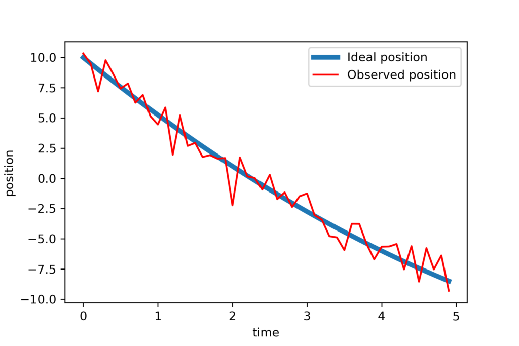
The vector positionNoisy is our noise corrupted position and the entries of this vector are $\mathbf{y}_{k}$ . We plot the noise-free and noisy position:

# verify the position vector by plotting the results
plotStep=numberTimeSteps//2
plt.plot(timeVector[0:plotStep],position[0:plotStep],linewidth=4, label='Ideal position')
plt.plot(timeVector[0:plotStep],positionNoisy[0:plotStep],'r', label='Observed position')
plt.xlabel('time')
plt.ylabel('position')
plt.legend()
plt.savefig('data.png',dpi=300)
plt.show()

The results are shown in the figure below.

Figure 2: Noise-free (ideal position) and noisy position measurements.

Next, we create a KalmanFilter object and simulate the Kalman filter equations:

#create a Kalman filter object 
KalmanFilterObject=KalmanFilter(x0,P0,A,B,C,Q,R)
inputValue=np.matrix([[0]])
# simulate online prediction
for j in np.arange(np.size(timeVector)):
    KalmanFilterObject.propagateDynamics(inputValue)
    KalmanFilterObject.computeAposterioriEstimate(positionNoisy[j])

KalmanFilterObject.estimates_aposteriori

The for loop iterates over the time vector. The call of the function KalmanFilterObject.propagateDynamics(inputValue) computes the step (18). On the other hand, the call of the function KalmanFilterObject.computeAposterioriEstimate(positionNoisy[j]) computes the step (19). We can obtain the computed estimates by executing this code line: KalmanFilterObject.estimates_aposteriori.

Finally, we can visualize the estimates by executing these code lines:

# extract the state estimates in order to plot the results
estimate1=[]
estimate2=[]
estimate3=[]    
for j in np.arange(np.size(timeVector)):
    estimate1.append(KalmanFilterObject.estimates_aposteriori[j][0,0])
    estimate2.append(KalmanFilterObject.estimates_aposteriori[j][1,0])
    estimate3.append(KalmanFilterObject.estimates_aposteriori[j][2,0])
    
# create vectors corresponding to the true values in order to plot the results
estimate1true=position
estimate2true=velocity
estimate3true=acceleration*np.ones(np.size(timeVector))


# plot the results
steps=np.arange(np.size(timeVector))
fig, ax = plt.subplots(3,1,figsize=(10,15))
ax[0].plot(steps,estimate1true,color='red',linestyle='-',linewidth=6,label='True value of position')
ax[0].plot(steps,estimate1,color='blue',linestyle='-',linewidth=3,label='Estimate of position')
ax[0].set_xlabel("Discrete-time steps k",fontsize=14)
ax[0].set_ylabel("Position",fontsize=14)
ax[0].tick_params(axis='both',labelsize=12)
#ax[0].set_yscale('log')
#ax[0].set_ylim(98,102)  
ax[0].grid()
ax[0].legend(fontsize=14)

ax[1].plot(steps,estimate2true,color='red',linestyle='-',linewidth=6,label='True value of velocity')
ax[1].plot(steps,estimate2,color='blue',linestyle='-',linewidth=3,label='Estimate of velocity')
ax[1].set_xlabel("Discrete-time steps k",fontsize=14)
ax[1].set_ylabel("Velocity",fontsize=14)
ax[1].tick_params(axis='both',labelsize=12)
#ax[0].set_yscale('log')
#ax[1].set_ylim(0,2)  
ax[1].grid()
ax[1].legend(fontsize=14)

ax[2].plot(steps,estimate3true,color='red',linestyle='-',linewidth=6,label='True value of acceleration')
ax[2].plot(steps,estimate3,color='blue',linestyle='-',linewidth=3,label='Estimate of acceleration')
ax[2].set_xlabel("Discrete-time steps k",fontsize=14)
ax[2].set_ylabel("Acceleration",fontsize=14)
ax[2].tick_params(axis='both',labelsize=12)
#ax[0].set_yscale('log')
#ax[1].set_ylim(0,2)  
ax[2].grid()
ax[2].legend(fontsize=14)

fig.savefig('plots.png',dpi=600)

As the result, we obtain the following graph

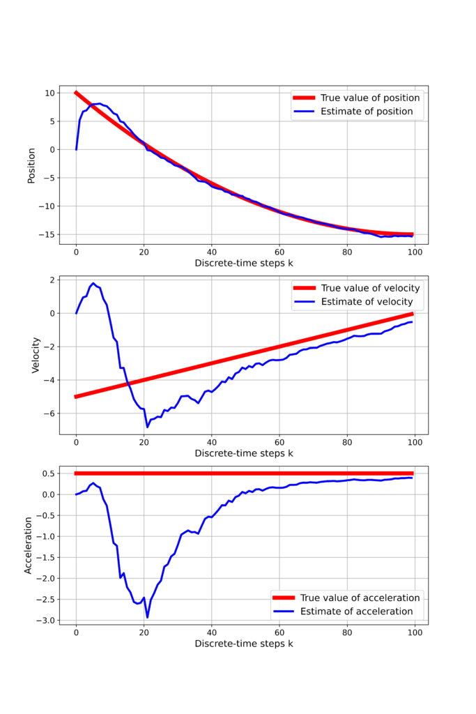
Figure 3: Computed estimates and the comparison.

From Figure 3 we can observe that all 3 states eventually converge to the true values.

Summary of the Kalman Filter Equations

Test Example

Object-oriented Python Implementation of the Kalman Filter

admin

You might also like

Easily Solve the Lyapunov Equation by Using the Kronecker Product – Detailed Explanation with Python Codes

Matrix Minor, Matrix Cofactor, Adjugate Matrix, and Formula for Matrix Inversion – Linear Algebra Tutorial

Solve Inverse Kinematics Problem in MATLAB