Extended Kalman Filter Tutorial With Example and Disciplined Python Code – PART II -Test Example and Python Codes – Fusion of Engineering, Control, Coding, Machine Learning, and Science

This is the second part of the tutorial on the extended (nonlinear) Kalman filter. In this tutorial, we explain how to implement the extended filter in Python. In the first tutorial part, we explained how to derive the extended Kalman filter. The YouTube videos accompanying this tutorial are given below. The GitHub page with the code used in this tutorial is given here.

The first part of the tutorial:

The second part of the tutorial

Test Example and Discretization

To test the performance of the extended Kalman filter, we consider a pendulum system. This is a classical dynamical system and if we use the programming analogy, this example can be seen as a “Hello World” example of control engineering and control theory. In our previous tutorial given over here, we derived an equation of motion and a state space model of the pendulum system. The state-space model has the following form

(1) $\begin{align*}\dot{\mathbf{x}}=\begin{bmatrix} \dot{x}_{1} \\ \dot{x}_{2} \end{bmatrix} = \begin{bmatrix} x_{2} \\ -\frac{g}{l} \sin(x_{1})\end{bmatrix}\end{align*}$

where $x_{1}$ is the angle of the pendulum, $x_{2}$ is the angular velocity, $g$ is the gravitational acceleration constant, and $l$ is the length of the pendulum. We assume that only the angle of the pendulum is directly measured. Consequently, the output equation is

(2) $\begin{align*}y=\begin{bmatrix} 1 & 0 \end{bmatrix}\begin{bmatrix} x_{1} \\ x_{2} \end{bmatrix}\end{align*}$

The model (1) is the continuous time form. Although we can develop the extended Kalman filter by directly using the continuous time form, the first part of this tutorial is based on the discrete-time system model. Consequently, in order to keep this second part of the tutorial consistent with the first one, we need to discretize the system (1).

The state-space model can be written in the general form

(3) $\begin{align*}\dot{\mathbf{x}}=\boldsymbol{\beta}\big(\mathbf{x} \big)\end{align*}$

where

(4) $\begin{align*}\boldsymbol{\beta}\big(\mathbf{x} \big) = \begin{bmatrix} x_{2} \\ -\frac{g}{l} \sin(x_{1})\end{bmatrix}\end{align*}$

We use the forward Euler discretization to approximate the first derivative

(5) $\begin{align*}\frac{\mathbf{x}_{k}-\mathbf{x}_{k-1}}{\Delta t} \approx \boldsymbol{\beta}(\mathbf{x} _{k-1})\end{align*}$

where $k$ is a discrete-time instant and $\Delta t$ is the discretization step size. From the last equation, we obtain

(6) $\begin{align*}\mathbf{x}_{k}\approx \mathbf{x}_{k-1} + \Delta t \cdot \boldsymbol{\beta}(\mathbf{x} _{k-1})\end{align*}$

By replacing the approximate equality sign with the strict equality, we obtain

(7) $\begin{align*}\mathbf{x}_{k}= \mathbf{x}_{k-1} + \Delta t \cdot \boldsymbol{\beta}(\mathbf{x} _{k-1})\end{align*}$

Next, by combining the expression for the function $\boldsymbol{\beta}(\cdot )$ that defined in (4) with the equation (7), we obtain

(8) $\begin{align*}\mathbf{x}_{k} = \begin{bmatrix} x_{1,k} \\ x_{2,k} \end{bmatrix} =\begin{bmatrix}x_{1,k-1}+\Delta t \cdot x_{2,k-1} \\ x_{2,k-1} -\Delta t \cdot \frac{g}{l} \sin(x_{1,k-1})\end{bmatrix}\end{align*}$

The last equation can be written in the compact form

(9) $\begin{align*}\mathbf{x}_{k}=\mathbf{f}\big(\mathbf{x}_{k-1} \big) \end{align*}$

where

(10) $\begin{align*}\mathbf{f}\big(\mathbf{x}_{k-1} \big) =\begin{bmatrix}x_{1,k-1}+\Delta t \cdot x_{2,k-1} \\ x_{2,k-1}-\Delta t \frac{g}{l}\sin(x_{1,k-1}) \end{bmatrix}\end{align*}$

Note that the function $\mathbf{f}()$ does not depend on time. Consequently, we do not have the index $k-1$ in its subscript (see the first part of this tutorial). By using the notation from the first part of this tutorial, we write the output equation (2) as follows

(11) $\begin{align*}\mathbf{y}_{k}=g\big(\mathbf{x}_{k} \big)\end{align*}$

where $g$ is a scalar output equation

(12) $\begin{align*}g\big(\mathbf{x}_{k} \big)=x_{1,k}\end{align*}$

Jacobian Matrix

Next, we need to compute the Jacobian matrices of the functions $\matbf{f}(\mathbf{x}_{k-1})$ and $\mathbf{g}\big(\mathbf{x}_{k} \big)$ . Let us first partition the matrix $\matbf{f}(\mathbf{x}_{k-1})$

(13) $\begin{align*}\matbf{f}(\mathbf{x}_{k-1})=\begin{bmatrix} f_{1}(\mathbf{x}_{k-1}) \\ f_{2}(\mathbf{x}_{k-1}) \end{bmatrix}\end{align*}$

where

(14) $\begin{align*}f_{1}(\mathbf{x}_{k-1}) =x_{1,k-1}+\Delta t \cdot x_{2,k-1} \\f_{2}(\mathbf{x}_{k-1})=x_{2,k-1}-\Delta t \frac{g}{l}\sin(x_{1,k-1})\end{align*}$

The Jacobian of the state vector function $\matbf{f}(\mathbf{x}_{k-1})$ is

(15) $\begin{align*}\frac{\partial \matbf{f}(\mathbf{x}_{k-1}) }{\partial \mathbf{x}_{k-1} }=\begin{bmatrix}\frac{\partial f_{1} }{\partial x_{1,k-1}} & \frac{\partial f_{1} }{\partial x_{2,k-1}} \\ \frac{\partial f_{2} }{\partial x_{1,k-1}} & \frac{\partial f_{2} }{\partial x_{2,k-1}} \end{bmatrix} =\begin{bmatrix} 1 & \Delta t \\ -\Delta t \frac{g}{l} \cos(x_{1,k-1}) & 1\end{bmatrix}\end{align*}$

The Jacobian matrix of the output function $g\big(\mathbf{x}_{k} \big)$ is

(16) $\begin{align*}\frac{\partial g(\mathbf{x}_{k})}{\partial \mathbf{x}_{k}}=\begin{bmatrix} \frac{\partial g(\mathbf{x}_{k})}{\partial \mathbf{x}_{1,k}} & \frac{\partial g(\mathbf{x}_{k})}{\partial \mathbf{x}_{2,k}} \end{bmatrix} =\begin{bmatrix}1 & 0 \end{bmatrix}\end{align*}$

On the basis of calculated Jacobians, we obtain the following matrices necessary for the extended Kalman filter implementation

(17) $\begin{align*}A_{k-1}=\frac{\partial \matbf{f}(\mathbf{x}_{k-1}) }{\partial \mathbf{x}_{k-1} }\Big|_{\mathbf{x}_{k-1}= \hat{\mathbf{x}}_{k-1}^{+}} = \begin{bmatrix} 1 & \Delta t \\ -\Delta t \frac{g}{l} \cos(x_{1,k-1}^{+}) & 1\end{bmatrix},\;\; C_{k}=\begin{bmatrix}1 & 0 \end{bmatrix}\end{align*}$

Python Code

The code presented in this tutorial are posted on the GitHub page. We wrote a Python class that implements the extended Kalman filter. First, for completeness, we present the complete class, and then we explain its functions and variables.

import numpy as np 

class ExtendedKalmanFilter(object):
    
    # x0 - initial guess of the state vector - this is the initial a posteriori estimate
    # P0 - initial guess of the covariance matrix of the state estimation error
    # Q  - covariance matrix of the process noise 
    # R  - covariance matrix of the measurement noise
    # dT - discretization period for the forward Euler method
    
    def __init__(self,x0,P0,Q,R,dT):
        
        # initialize vectors and matrices
        self.x0=x0
        self.P0=P0
        self.Q=Q
        self.R=R
        self.dT=dT
        
        # model parameters
        # gravitational constant
        self.g=9.81
        # length of the pendulum 
        self.l=1
        
        # this variable is used to track the current time step k of the estimator 
        # after every measurement arrives, this variables is incremented for +1 
        self.currentTimeStep=0
        
        # this list is used to store the a posteriori estimates hat{x}_k^{+} starting from the initial estimate 
        # note: the list starts from hat{x}_0^{+}=x0 - where x0 is an initial guess of the estimate provided by the user
        self.estimates_aposteriori=[]
        self.estimates_aposteriori.append(x0)
        
        # this list is used to store the a apriori estimates hat{x}_k^{-} starting from hat{x}_1^{-}
        # note: hat{x}_0^{-} does not exist, that is, the list starts from the time index 1
        self.estimates_apriori=[]
        
        # this list is used to store the a posteriori estimation error covariance matrices P_k^{+}
        # note: the list starts from P_0^{+}=P0, where P0 is the initial guess of the covariance provided by the user
        self.estimationErrorCovarianceMatricesAposteriori=[]
        self.estimationErrorCovarianceMatricesAposteriori.append(P0)
        
        # this list is used to store the a priori estimation error covariance matrices P_k^{-}
        # note: the list starts from P_1^{-}, that is, it starts from the time index 1
        self.estimationErrorCovarianceMatricesApriori=[]
        
        # this list is used to store the Kalman gain matrices K_k
        self.gainMatrices=[]
         
        # this list is used to store prediction errors error_k=y_k-self.outputEquation(x_k^{-})
        self.errors=[]
    
    
    # here is the continuous state-space model
    # inputs:
    #       x - state vector 
    #       t - time
    # NOTE THAT WE ARE NOT USING time since the dynamics is time invariant
    # output: 
    #       dxdt - the value of the state function (derivative of x)
    def stateSpaceContinuous(self,x,t):
        dxdt=np.array([[x[1,0]],[-(self.g/self.l)*np.sin(x[0,0])]])
        return dxdt
    
    # this function defines the discretized state-space model 
    # we use the forward Euler discretization 
    # input: 
    #       x_k   - current state x_{k}
    # output:
    #       x_kp1 - state propagated in time x_{k+1}
    def discreteTimeDynamics(self,x_k):
        # note over here that we are not using "self.currentTimeStep*self.DT" since the dynamics is time invariant
        # however, you might need to use this argument if your dynamics is time varying
        x_kp1=x_k+self.dT*self.stateSpaceContinuous(x_k,self.currentTimeStep*self.dT)
        return x_kp1
    
    # this function returns the Jacobian of the discrete-time state equation 
    # evaluated at x_k
    # That is, it returns the matrix A
    # input: 
    #       x_k - state 
    # output: 
    #       A - the Jacobian matrix of the state equation with respect to state
    def jacobianStateEquation(self,x_k):
        A=np.zeros(shape=(2,2))
        A[0,0]=1
        A[0,1]=self.dT
        A[1,0]=-self.dT*(self.g/self.l)*np.cos(x_k[0,0])
        A[1,1]=1
        return A
    
    # this function returns the Jacobian of the output equation 
    # evaluated at x_k
    # That is, it returns the matrix C
    # Note that since in the case of the pendulum the output is a linear function 
    # and consequently, we actually do not use x_k
    # however, in the case of nonlinear output functions we need x_k
    # input: 
    #      x_k - state 
    # output: 
    #      C   - the Jacobian matrix of the output equation with respect to state
    def jacobianOutputEquation(self,x_k):
        C=np.zeros(shape=(1,2))
        C[0,0]=1
        return C
    
    # this is the output equation
    # input: 
    #       x_k - state
    # output: 
    #       x_k[0]- output value at the current state
    def outputEquation(self,x_k):
        return x_k[0]
    
    # this function propagates x_{k-1}^{+} through the model to compute x_{k}^{-}
    # this function also propagates P_{k-1}^{+} through the time-covariance model to compute P_{k}^{-}
    # at the end, this function increments the time index self.currentTimeStep for +1
     
    def propagateDynamics(self):
        # propagate the a posteriori estimate to compute the a priori estimate
        xk_minus=self.discreteTimeDynamics(self.estimates_aposteriori[self.currentTimeStep])
        # linearize the dynamics at the a posteriori estimate 
        Akm1=self.jacobianStateEquation(self.estimates_aposteriori[self.currentTimeStep])
        # propagate the a posteriori covariance matrix in time to compute the a priori covariance
        Pk_minus=np.matmul(np.matmul(Akm1,self.estimationErrorCovarianceMatricesAposteriori[self.currentTimeStep]),Akm1.T)+self.Q
        
        # memorize the computed values and increment the time step
        self.estimates_apriori.append(xk_minus)
        self.estimationErrorCovarianceMatricesApriori.append(Pk_minus)
        self.currentTimeStep=self.currentTimeStep+1
    
    # this function computes the a posteriori estimate by using the measurements
    # this function should be called after propagateDynamics() because the time step should be increased and states and covariances should be propagated         
    # input:
    #       currentMeasurement - measurement at the time step k
    def computeAposterioriEstimate(self,currentMeasurement):
                
        
        # linearize the output equation at the a priori estimate for the time step k
        Ck=self.jacobianOutputEquation(self.estimates_apriori[self.currentTimeStep-1]) 
        
        # compute the Kalman gain matrix
        # keep in mind that the a priori indices start from k=1, that is why we index a priori quantities with "self.currentTimeStep-1"
        Smatrix= self.R+np.matmul(np.matmul(Ck,self.estimationErrorCovarianceMatricesApriori[self.currentTimeStep-1]),Ck.T)
        # Kalman gain matrix
        Kk=np.matmul(self.estimationErrorCovarianceMatricesApriori[self.currentTimeStep-1],np.matmul(Ck.T,np.linalg.inv(Smatrix)))
        
        # update the estimate
        # prediction error
        error_k=currentMeasurement-self.outputEquation(self.estimates_apriori[self.currentTimeStep-1])
        # a posteriori estimate
        xk_plus=self.estimates_apriori[self.currentTimeStep-1]+np.matmul(Kk,np.array([error_k]))
        
        # update the covariance matrix
        # a posteriori covariance matrix update 
        IminusKkC=np.eye(self.x0.shape[0])-np.matmul(Kk,Ck)
        Pk_plus=np.matmul(IminusKkC,np.matmul(self.estimationErrorCovarianceMatricesApriori[self.currentTimeStep-1],IminusKkC.T))+np.matmul(Kk,np.matmul(self.R,Kk.T))
        
        # update the lists that store the vectors and matrices
        # Kalman gain matrix
        self.gainMatrices.append(Kk)
        # errors
        self.errors.append(error_k)
        # a posteriori estimates
        self.estimates_aposteriori.append(xk_plus)
        # a posteriori covariance matrix
        self.estimationErrorCovarianceMatricesAposteriori.append(Pk_plus)

First, we define the __init__() function that is repeated over here for completness

def __init__(self,x0,P0,Q,R,dT):
        
        # initialize vectors and matrices
        self.x0=x0
        self.P0=P0
        self.Q=Q
        self.R=R
        self.dT=dT
        
        # model parameters
        # gravitational constant
        self.g=9.81
        # length of the pendulum 
        self.l=1
        
        # this variable is used to track the current time step k of the estimator 
        # after every measurement arrives, this variables is incremented for +1 
        self.currentTimeStep=0
        
        # this list is used to store the a posteriori estimates hat{x}_k^{+} starting from the initial estimate 
        # note: the list starts from hat{x}_0^{+}=x0 - where x0 is an initial guess of the estimate provided by the user
        self.estimates_aposteriori=[]
        self.estimates_aposteriori.append(x0)
        
        # this list is used to store the a apriori estimates hat{x}_k^{-} starting from hat{x}_1^{-}
        # note: hat{x}_0^{-} does not exist, that is, the list starts from the time index 1
        self.estimates_apriori=[]
        
        # this list is used to store the a posteriori estimation error covariance matrices P_k^{+}
        # note: the list starts from P_0^{+}=P0, where P0 is the initial guess of the covariance provided by the user
        self.estimationErrorCovarianceMatricesAposteriori=[]
        self.estimationErrorCovarianceMatricesAposteriori.append(P0)
        
        # this list is used to store the a priori estimation error covariance matrices P_k^{-}
        # note: the list starts from P_1^{-}, that is, it starts from the time index 1
        self.estimationErrorCovarianceMatricesApriori=[]
        
        # this list is used to store the Kalman gain matrices K_k
        self.gainMatrices=[]
         
        # this list is used to store prediction errors error_k=y_k-self.outputEquation(x_k^{-})
        self.errors=[]

The input variables are

“x0” is the initial guess of the a posteriori state $\mathbf{x}_{0}^{+}$ that is selected by the user.
“P0” is the initial guess of the a posteriori covariance matrix $P_{0}^{+}$ that is selected by the user.
“Q” is the covariance matrix of the process noise.
“R” is the covariance matrix of the measurement noise.
“dT” is the discretization time constant $\Delta t$ in (5).

On the code lines 22 and 24 we define the constants $g$ and $l$ . Next, we explain the variables that are created and initialized by this function

“self.currentTimeStep” is used to memorize the current time step $k$ .
“self.estimates_aposteriori” is the list used to store the a posteriori estimates $\mathbf{x}_{k-1}^{+}$
“self.estimates_apriori” is the list used to store the a priori estimates $\mathbf{x}_{k}^{-}$
“self.estimationErrorCovarianceMatricesAposteriori” is the list used to store $P_{k-1}^{+}$
“self.estimationErrorCovarianceMatricesApriori” is the list used to store $P_{k}^{-}$
“self.gainMatrices” is the list used to store the gain matrices $K_{k}$
“self.errors” is the list used to store the errors
(18) $\begin{align*}\mathbf{y}_{k}-g\big(\mathbf{x}_{k}^{-} \big)\end{align*}$

The right-hand side of the continuous time state equation (1) is defined by

    def stateSpaceContinuous(self,x,t):
        dxdt=np.array([[x[1,0]],[-(self.g/self.l)*np.sin(x[0,0])]])
        return dxdt

The discrete-time dynamics (8) is shifted one step in time, and is defined by the following function

    def discreteTimeDynamics(self,x_k):
        # note over here that we are not using "self.currentTimeStep*self.DT" since the dynamics is time invariant
        # however, you might need to use this argument if your dynamics is time varying
        x_kp1=x_k+self.dT*self.stateSpaceContinuous(x_k,self.currentTimeStep*self.dT)
        return x_kp1

The Jacobian matrix (15) of the state equation is defined by

    def jacobianStateEquation(self,x_k):
        A=np.zeros(shape=(2,2))
        A[0,0]=1
        A[0,1]=self.dT
        A[1,0]=-self.dT*(self.g/self.l)*np.cos(x_k[0,0])
        A[1,1]=1
        return A

The Jacobian matrix (16) of the output equation is defined by

    def jacobianOutputEquation(self,x_k):
        C=np.zeros(shape=(1,2))
        C[0,0]=1
        return C

The output equation (2) is defined by

    def outputEquation(self,x_k):
        return x_k[0]

The first step of the Kalman filter (see the first part of the tutorial) is to propagate a posteriori estimate and covariance matrix through the dynamics:

(19) $\begin{align*}\hat{\mathbf{x}}_{k}^{-}=\mathbf{f}_{k-1}\big(\hat{\mathbf{x}}_{k-1}^{+}, \mathbf{u}_{k-1}= \mathbf{u}_{k-1}^{*} \big) \\P_{k}^{-}=A_{k-1}P_{k-1}^{+}A_{k-1}^{T}+Q_{k-1}\end{align*}$

This is achieved by the following function

    def propagateDynamics(self):
        # propagate the a posteriori estimate to compute the a priori estimate
        xk_minus=self.discreteTimeDynamics(self.estimates_aposteriori[self.currentTimeStep])
        # linearize the dynamics at the a posteriori estimate 
        Akm1=self.jacobianStateEquation(self.estimates_aposteriori[self.currentTimeStep])
        # propagate the a posteriori covariance matrix in time to compute the a priori covariance
        Pk_minus=np.matmul(np.matmul(Akm1,self.estimationErrorCovarianceMatricesAposteriori[self.currentTimeStep]),Akm1.T)+self.Q
        
        # memorize the computed values and increment the time step
        self.estimates_apriori.append(xk_minus)
        self.estimationErrorCovarianceMatricesApriori.append(Pk_minus)
        self.currentTimeStep=self.currentTimeStep+1

Note that in this step we also update the appropriate lists and the current time step $k$ .

In the second step, we calculate

(20) $\begin{align*}K_{k}=P_{k}^{-}C_{k}^{T}\big(C_{k}P_{k}^{-}C_{k}^{T}+R_{k} \big)^{-1}\end{align*}$

(21) $\begin{align*}\hat{\mathbf{x}}_{k}^{+} & =\hat{\mathbf{x}}_{k}^{-}+K_{k}\big(\mathbf{y}_{k}- \mathbf{g}_{k}\big(\hat{\mathbf{x}}_{k}^{-} \big) \big) \end{align*}$

(22) $\begin{align*}P_{k}^{+}=\big(I-K_{k}C_{k} \big)P_{k}^{-}\big(I-K_{k}C_{k} \big)^{T}+K_{k}R_{k}K_{k}^{T}\end{align*}$

These steps are implemented by the following function

 def computeAposterioriEstimate(self,currentMeasurement):
                
        
        # linearize the output equation at the a priori estimate for the time step k
        Ck=self.jacobianOutputEquation(self.estimates_apriori[self.currentTimeStep-1]) 
        
        # compute the Kalman gain matrix
        # keep in mind that the a priori indices start from k=1, that is why we index a priori quantities with "self.currentTimeStep-1"
        Smatrix= self.R+np.matmul(np.matmul(Ck,self.estimationErrorCovarianceMatricesApriori[self.currentTimeStep-1]),Ck.T)
        # Kalman gain matrix
        Kk=np.matmul(self.estimationErrorCovarianceMatricesApriori[self.currentTimeStep-1],np.matmul(Ck.T,np.linalg.inv(Smatrix)))
        
        # update the estimate
        # prediction error
        error_k=currentMeasurement-self.outputEquation(self.estimates_apriori[self.currentTimeStep-1])
        # a posteriori estimate
        xk_plus=self.estimates_apriori[self.currentTimeStep-1]+np.matmul(Kk,np.array([error_k]))
        
        # update the covariance matrix
        # a posteriori covariance matrix update 
        IminusKkC=np.eye(self.x0.shape[0])-np.matmul(Kk,Ck)
        Pk_plus=np.matmul(IminusKkC,np.matmul(self.estimationErrorCovarianceMatricesApriori[self.currentTimeStep-1],IminusKkC.T))+np.matmul(Kk,np.matmul(self.R,Kk.T))
        
        # update the lists that store the vectors and matrices
        # Kalman gain matrix
        self.gainMatrices.append(Kk)
        # errors
        self.errors.append(error_k)
        # a posteriori estimates
        self.estimates_aposteriori.append(xk_plus)
        # a posteriori covariance matrix
        self.estimationErrorCovarianceMatricesAposteriori.append(Pk_plus)

This function also updates the appropriate lists. This class should be saved in the file called “ExtendedKalmanFilter.py”

Next, we present the driver code that explains how to use this class. The following code lines import the necessary libraries, simulate the pendulum dynamics by using the odeint() function and the forward Euler method. This is done to quantify the model differences between very precise simulation of the dynamics and simulation by using the forward Euler method that is used to develop the dynamics. Note that we are using the simulations obtained by using the odeint() function as “true” measurements. In this tutorial, we explain how to simulate the dynamics by using the odeint() function.

import numpy as np
import matplotlib.pyplot as plt

# this function is used to integrate the dynamics
from scipy.integrate import odeint
# in this class we implement the extended Kalman filter
from ExtendedKalmanFilter import ExtendedKalmanFilter

# discretization time step
# it is used for both integration of the pendulum differential equation and for
# forward Euler method discretization
deltaTime=0.01
# initial condition for generating the simulation data 
x0=np.array([np.pi/3,0.2])

# time steps for simulation
simulationSteps=400
# total simulation time 
totalSimulationTimeVector=np.arange(0,simulationSteps*deltaTime,deltaTime)

# this state-space model defines the continuous dynamics of the pendulum
# this function is passed as an argument of the odeint() function for integrating (solving) the dynamics 
def stateSpaceModel(x,t):
    g=9.81
    # 
    l=1
    dxdt=np.array([x[1],-(g/l)*np.sin(x[0])])
    return dxdt

# here we integrate the dynamics
# the output: "solutionOde" contains time series of the angle and angular velocity 
# these time series represent the time series of the true state that we want to estimate
solutionOde=odeint(stateSpaceModel,x0,totalSimulationTimeVector)
 
# uncomment this if you want to plot the simulation results 
#plt.plot(totalSimulationTimeVector, solutionOde[:, 0], 'b', label='x1')
#plt.plot(totalSimulationTimeVector, solutionOde[:, 1], 'g', label='x2')
#plt.legend(loc='best')
#plt.xlabel('time')
#plt.ylabel('x1(t), x2(t)')
#plt.grid()
#plt.savefig('simulation.png',dpi=600)
#plt.show()

# here we compare the forward Euler discretization with the odeint()
# this is important for evaluating the accuracy of the forward Euler method 

forwardEulerState=np.zeros(shape=(simulationSteps,2))
# set the initial states to match the initial state used in the odeint()
forwardEulerState[0,0]=x0[0]
forwardEulerState[0,1]=x0[1]

# propagate the forward Euler dynamics
for timeIndex in range(simulationSteps-1):
    forwardEulerState[timeIndex+1,:]=forwardEulerState[timeIndex,:]+deltaTime*stateSpaceModel(forwardEulerState[timeIndex,:],timeIndex*deltaTime)
    
# plot the comparison results
plt.plot(totalSimulationTimeVector, solutionOde[:, 0], 'r', linewidth=3, label='Angle - ODEINT')
plt.plot(totalSimulationTimeVector, forwardEulerState[:, 0], 'b', linewidth=2, label='Angle- Forward Euler')
plt.legend(loc='best')
plt.xlabel('time [s]')
plt.ylabel('Angle-x1(t)')
plt.grid()
plt.savefig('comparison.png',dpi=600)
plt.show()

This code produces the following graph

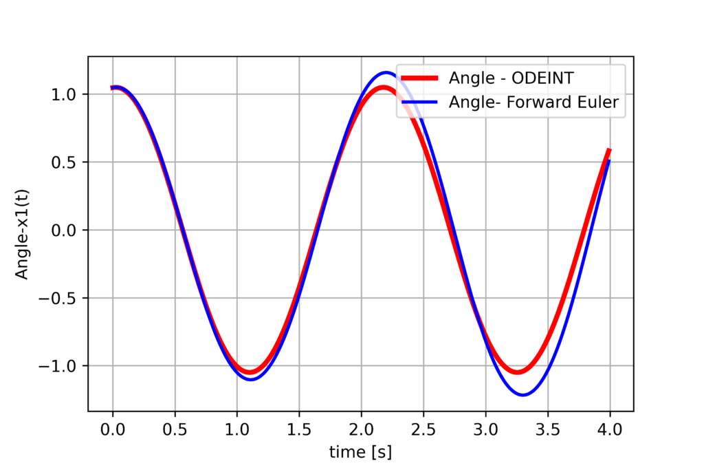
Figure 1: Comparison of the odeint() integration with the forward Euler discretization.

We can see that the forward Euler method sufficiently accurately discretizes the dynamics.

Next, we select the initial estimate and the initial covariance matrix, simulate the Kalman filter, and plot the results. This is done by using the following code

#create the Kalman filter object 
# this is an initial guess of the state estimate
x0guess=np.zeros(shape=(2,1))
x0guess[0]=x0[0]+4*np.random.randn()
x0guess[1]=x0[1]+4*np.random.randn()

# initial value of the covariance matrix
P0=10*np.eye(2,2)
# discretization stpe
dT=deltaTime
# process noise covariance matrix
# note that we do not have the process noise
Q=0.0001*np.eye(2,2)
# measurement noise covariance matrix
# note that we do not have measurement noise in this simulation 
# see driverCodeNoise.py for the performance when the measurement noise
# is affecting the outputs
R=np.array([[0.0001]])

# create the extended Kalman filter object
KalmanFilterObject=ExtendedKalmanFilter(x0guess,P0,Q,R,dT)


# simulate the extended Kalman filter 
for j in range(simulationSteps-1):
    # TWO STEPS
    # (1) propagate a posteriori estimate and covariance matrix
    KalmanFilterObject.propagateDynamics()
    
    # (2) take into account the current measurement and 
    # compute the a posteriori estimate and covarance matrix
    # note that we use the exact solution of the differential 
    # equations as measurements
    # note also that we only measure the angle of the pendulum
    KalmanFilterObject.computeAposterioriEstimate(solutionOde[j, 0])

# Estimates
#KalmanFilterObject.estimates_aposteriori
# Covariance matrices
#KalmanFilterObject.estimationErrorCovarianceMatricesAposteriori
# Kalman gain matrices
#KalmanFilterObject.gainMatrices.append(Kk)
# errors
#KalmanFilterObject.errors.append(error_k)

# extract the state estimates in order to plot the results
estimateAngle=[]
estimateAngularVelocity=[]
for j in np.arange(np.size(totalSimulationTimeVector)):
    estimateAngle.append(KalmanFilterObject.estimates_aposteriori[j][0,0])
    estimateAngularVelocity.append(KalmanFilterObject.estimates_aposteriori[j][1,0])
   
    
# create vectors corresponding to the true values in order to plot the results
trueAngle=solutionOde[:,0]
trueAngularVelocity=solutionOde[:,1]


# plot the results
steps=np.arange(np.size(totalSimulationTimeVector))
fig, ax = plt.subplots(2,1,figsize=(10,15))
ax[0].plot(steps,trueAngle,color='red',linestyle='-',linewidth=6,label='True angle')
ax[0].plot(steps,estimateAngle,color='blue',linestyle='-',linewidth=3,label='Estimate of angle')
ax[0].set_xlabel("Discrete-time steps k",fontsize=14)
ax[0].set_ylabel("Angle",fontsize=14)
ax[0].tick_params(axis='both',labelsize=12)
ax[0].grid()
ax[0].legend(fontsize=14)

ax[1].plot(steps,trueAngularVelocity,color='red',linestyle='-',linewidth=6,label='True angular velocity')
ax[1].plot(steps,estimateAngularVelocity,color='blue',linestyle='-',linewidth=3,label='Angular velocity estimate')
ax[1].set_xlabel("Discrete-time steps k",fontsize=14)
ax[1].set_ylabel("Angular Velocity",fontsize=14)
ax[1].tick_params(axis='both',labelsize=12)
ax[1].grid()
ax[1].legend(fontsize=14)
fig.savefig('estimationResults.png',dpi=600)

The results are shown below.

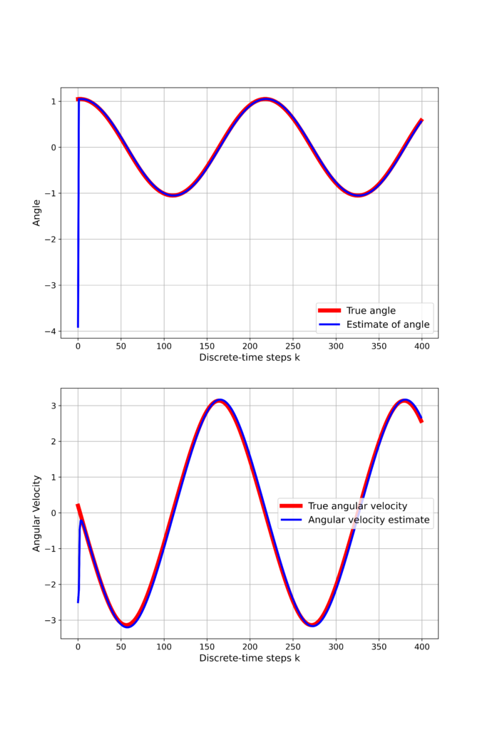
We can observe that the initial guess quickly converges to the true system states. The Kalman filter is created as follows

KalmanFilterObject=ExtendedKalmanFilter(x0guess,P0,Q,R,dT)

The Kalman filter is simulated by using the following loop

for j in range(simulationSteps-1):
    # TWO STEPS
    # (1) propagate a posteriori estimate and covariance matrix
    KalmanFilterObject.propagateDynamics()
    
    # (2) take into account the current measurement and 
    # compute the a posteriori estimate and covarance matrix
    # note that we use the exact solution of the differential 
    # equations as measurements
    # note also that we only measure the angle of the pendulum
    KalmanFilterObject.computeAposterioriEstimate(solutionOde[j, 0])

First, we propagate the dynamics, and then we compute the a posteriori state estimates by using the measurements.

Test Example and Discretization

Jacobian Matrix

Python Code

admin

You might also like

Contour Detection in OpenCV (Python) – OpenCV Tutorial in Python

Explanation of Python’s Meshgrid Function (Numpy) and 3D Plotting in Python

Homogeneous Transformation: Rotation and Translation