Explanation of Python’s Meshgrid Function (Numpy) and 3D Plotting in Python

In this post, we explain Python’s meshgrid function which is very useful for creating 3D plots. By reading this post, you will learn how to

1. Create a meshgrid
2. Use meshgrid to plot 3D functions in Python by using contourf(), plot_surface(), and contour3D() functions.

The YouTube video accompanying this post is given here:

The following code lines import the necessary libraries and create meshgrid matrices X and Y:

# -*- coding: utf-8 -*-
"""
Created on Thu Jun 16 22:27:26 2022

@author: ahaber
"""

from mpl_toolkits import mplot3d
import matplotlib.pyplot as plt
import numpy as np

# demonstration 

x=np.linspace(0,5,6)
y=np.linspace(0,5,6)

X, Y = np.meshgrid(x,y)

X[0,:]
Y[0,:]

for pair in zip(X[0,:],Y[0,:]):
    print(pair)

First, we import “from mpl_toolkits import mplot3d”. mplot3d toolkit that is included with Matplotlib, enables 3D plotting (for more details, see the text below). The vectors “x” and “y” contain entries starting from 0 to 5. Then the code line “X, Y = np.meshgrid(x,y)”, creates two matrices X and Y. These matrices have the following structure:

X=array([[0., 1., 2., 3., 4., 5.],
[0., 1., 2., 3., 4., 5.],
[0., 1., 2., 3., 4., 5.],
[0., 1., 2., 3., 4., 5.],
[0., 1., 2., 3., 4., 5.],
[0., 1., 2., 3., 4., 5.]])

 Y=array([[0., 0., 0., 0., 0., 0.],
[1., 1., 1., 1., 1., 1.],
[2., 2., 2., 2., 2., 2.],
[3., 3., 3., 3., 3., 3.],
[4., 4., 4., 4., 4., 4.],
[5., 5., 5., 5., 5., 5.]])

These two matrices define a grid of points in the Cartesian plane. The coordinates of the points are (X[0,0],Y[0,0]),(X[0,1],Y[0,1]),(X[0,2],Y[0,2]),…,(X[i,j],Y[i,j]), where X[i,j] is the (i,j) entry of the matrix X, and where Y[i,j] is the (i,j) entry of the matrix Y. The grid is illustrated in the figure below.

We can get some of the coordinate pairs by typing

for pair in zip(X[0,:],Y[0,:]):
    print(pair)

These code lines produce

(0.0, 0.0)
(1.0, 0.0)
(2.0, 0.0)
(3.0, 0.0)
(4.0, 0.0)
(5.0, 0.0)

These points correspond to the points in the first row in Fig. 1.

Next, we explain how meshgrid function can be used to visualize 3D functions in Python.

First, we redefine the coordinates and define the parabolic function

# plotting
x=np.linspace(-5,5,11)
y=np.linspace(-5,5,11)

X, Y = np.meshgrid(x,y)
Z= X**2+Y**2

A few comments are in order. We defined the parabolic function:

(1)  

The Python code for defining this function is: Z= X**2+Y**2. Since, X and Y are matrices, the expressions X**2 and Y**2 are applied element-wise. Similarly, the addition X**2+Y**2 is applied element-wise. This means that Z[i,j]=X[i,j]**2 + Y[i,j]**2.

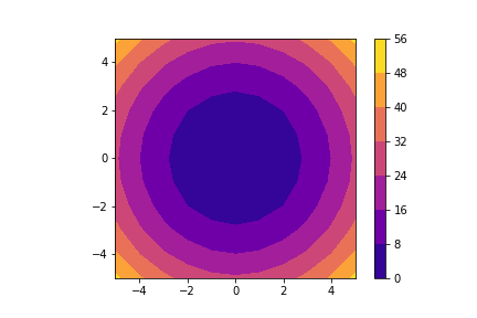
There are at least 3 ways for visualizing the 3D functions in Python. The first approach is to use contourf() function:

fig=plt.figure()
plt.contourf(X,Y,Z,cmap='plasma')
plt.axis('scaled')
plt.colorbar()
plt.savefig('contour1.png')
plt.show()

These code lines produce the following graph:

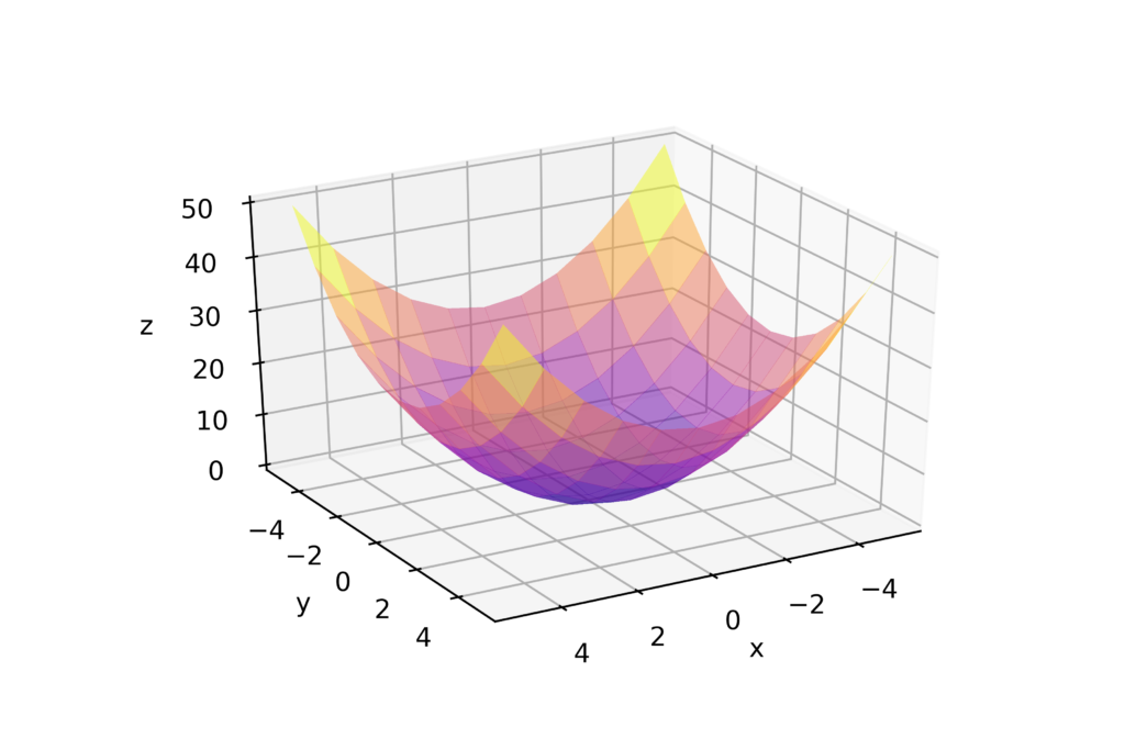
The second approach is to use the function plot_surface():

fig = plt.figure()
ax = plt.axes(projection='3d')
ax.plot_surface(X, Y, Z, cmap="plasma", linewidth=0, antialiased=False, alpha=0.5)
ax.set_xlabel('x')
ax.set_ylabel('y')
ax.set_zlabel('z');
# rotation
ax.view_init(30, 60)
plt.savefig('3Dplot1.png',dpi=600)
plt.show()

A few comments are in order. Code line 2 is used to set the 3D plotting mode. The prerequisite for using this approach is to import the following module:

from mpl_toolkits import mplot3d

We create the plot by calling the function “plot_surface(X, Y, Z, cmap=”plasma”, linewidth=0, antialiased=False, alpha=0.5)”. The first two arguments are X and Y matrices created by meshgrid() functions. The third argument is the Z value. Code line 8 is used is to set the rotation of the view in order to better visualize the plot. These code lines produce the following graph

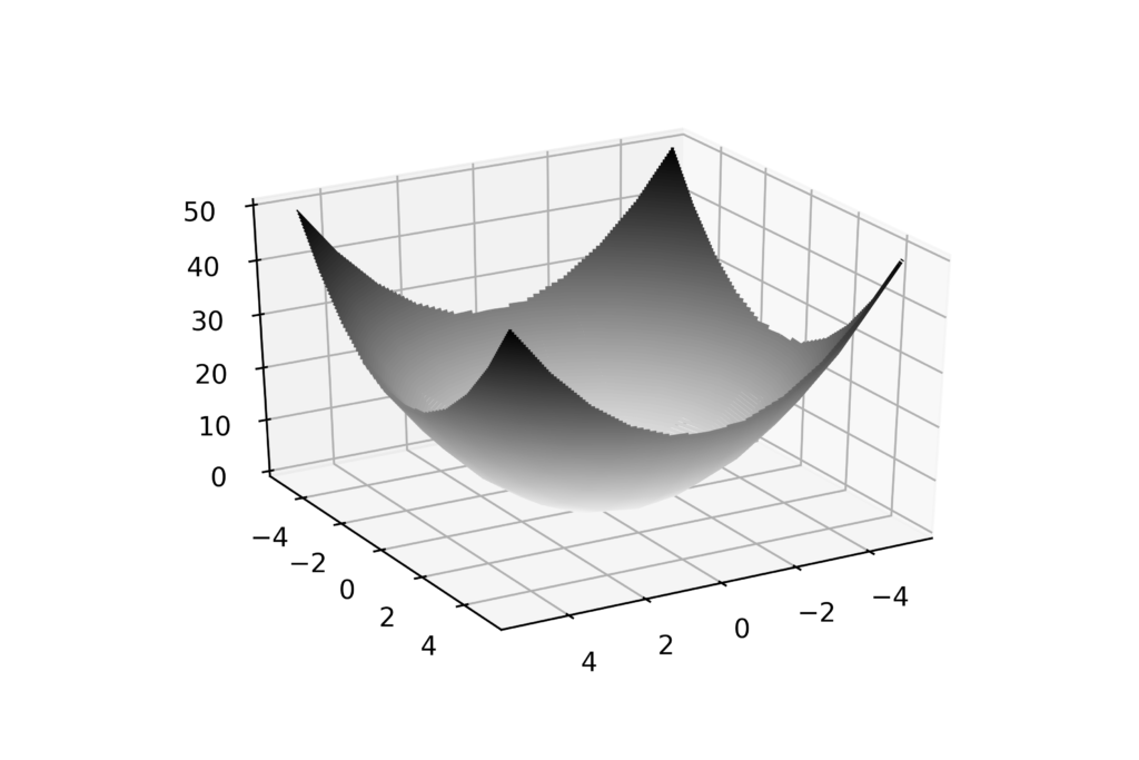
The next approach for creating the plot is to use the function contour3D() function. This approach creates the 3D contour plot:

fig = plt.figure()
ax = plt.axes(projection='3d')
ax.contour3D(X, Y, Z, 100, cmap='binary')
ax.view_init(30, 60)
plt.savefig('3Dplot2.png',dpi=600)
plt.show()

The code is self-explanatory. These code lines produce the following plot