Explanation of Meshgrid Function in MATLAB and 3D Plotting Using Mesh, Surf, and Surfl Functions

In this post, we explain how to

1.) Define a mesh in MATLAB by using the meshgrid function
2.) Use meshgrid function to create 3D plots by using mesh, surf, and surfl functions

The YouTube vidoe accompanying this post is given here

The following code lines create a pair of meshgrid matrices:

% basic illustration of the meshgrid function

x=0:1:5
y=0:1:5

[X,Y]=meshgrid(x,y)

X
Y

These code lines produce two matrices

X =

     0     1     2     3     4     5
     0     1     2     3     4     5
     0     1     2     3     4     5
     0     1     2     3     4     5
     0     1     2     3     4     5
     0     1     2     3     4     5

Y =

     0     0     0     0     0     0
     1     1     1     1     1     1
     2     2     2     2     2     2
     3     3     3     3     3     3
     4     4     4     4     4     4
     5     5     5     5     5     5

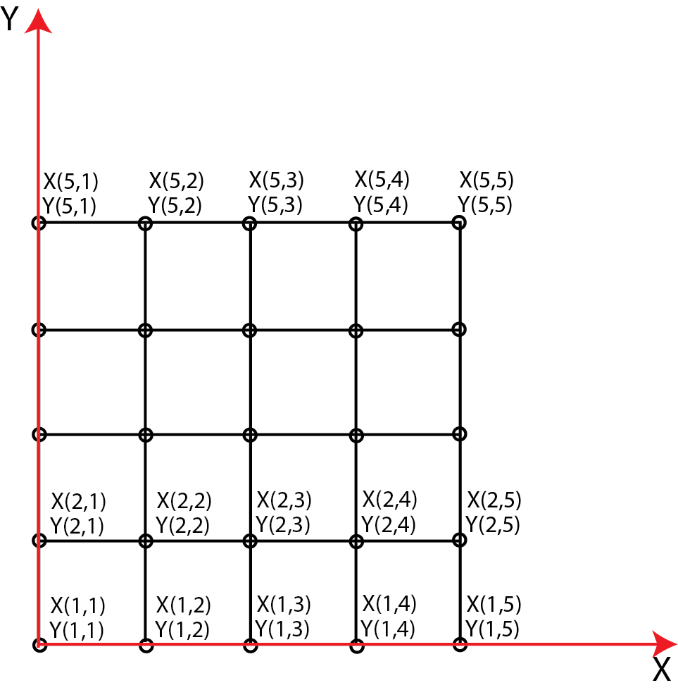
These two matrices define a grid of points. Before we explain this in more detail, let us first explain the code. First, we define two vectors x and y. These vectors separately define the x and y coordinates of points and limits of the grid. In our case, the grid will start from x=0 on the x-axis and it will end at x=5. We have a step of 1 between points. Similarly, the grid will start from y=0 on the y axis and it will end at y=5. The function meshgrid(x,y) takes the vectors x and y as inputs and produces two matrices X and Y. These matrices contain the coordinates of points in the Cartesian x-y plane that define the grid. The points are defined by ( X(1,1),Y(1,1) ), ( X(1,2),Y(1,2) ), ( X(1,3),Y(1,3) ), . . ., ( X(5,5),Y(5,5) ), where X(i,j) and Y(i,j) are the (i,j) entries of the matrix X and Y, respectively. The grid of points is shown in the figure below.

Next, we explain how to use the meshgrid function to create 3D plots of functions. First, we redefine the meshgrid

% redefine the meshgrid in order to plot a parabolic function

x=-5:0.5:5
y=-5:0.5:5

[X,Y]=meshgrid(x,y)

We define a parabolic function:

(1)  

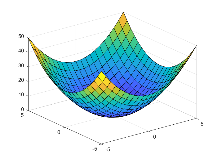
The parabolic function can be defined in MATLAB and plotted by using the following code lines

% parabolic function
Z1=X.^2+Y.^2

% plot using surf function
surf(X,Y,Z1)

The notation X.^2 means that we square every entry of the matrix X. The plot is shown below

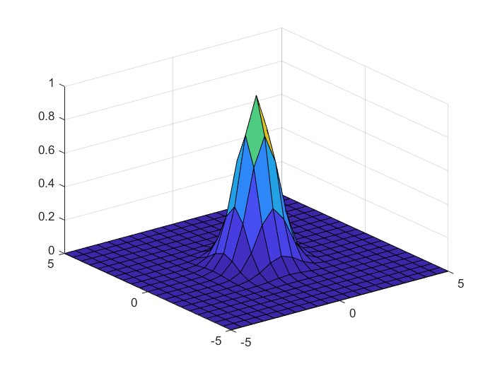
The function:

(2)  

can be plotted as follows

% another function 

Z2=exp(-X.^2-Y.^2)
surf(X,Y,Z2)

The resulting plot is shown below

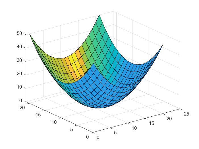
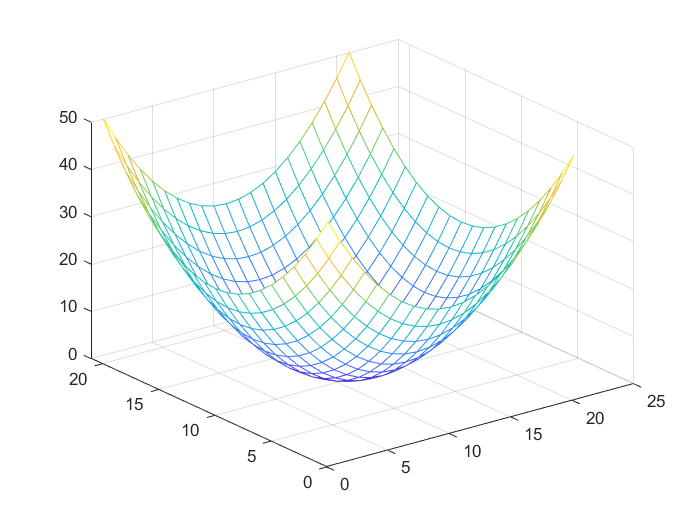
We can also use the mesh function to obtain 3D plots.

% plot using mesh function 

mesh(Z1)

The plot is given in the figure below.

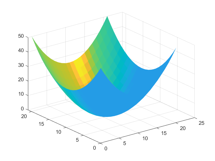
We can also use surfl function to obtain 3D plots:

% plot using surfl

surfl(Z1)
shading flat

surfl(Z1)
shading faceted

We use two methods of shading: “flat” and “facet”. The resulting plots are given below.