In this post, we provide a short introduction to the method of least squares. This method serves as the basis of many estimation and control algorithms. Consequently, every engineer, as well as other scientists, should have a working knowledge and basic understanding of this important method. In our next post, we will explain how to implement this method in C++ and Python. Also, in our future posts, we will explain how to recursively implement the least-squares method. A YouTube video accompanying this post is given below.
In the sequel, we present the problem formulation. Let us assume that we want to estimate a set of scalar variables: ![]() . However, all we have are the noisy observed (measured) variables
. However, all we have are the noisy observed (measured) variables ![]() , where in the general case
, where in the general case ![]() (basic engineering intuition tells us that we need to have more measurements than unknowns, that is the main reason why
(basic engineering intuition tells us that we need to have more measurements than unknowns, that is the main reason why ![]() ).
).
Let us assume that the observed variables are related to the set of scalar variables that we want to estimate via the following linear model
(1) 
where ![]() are scalars and
are scalars and ![]() is the measurement noise. Here it should be emphasized that the noise term is not known. All we can know are the statistical properties of the noise that can be estimated from the data. We assume that the measurement noise is zero mean and that
is the measurement noise. Here it should be emphasized that the noise term is not known. All we can know are the statistical properties of the noise that can be estimated from the data. We assume that the measurement noise is zero mean and that
(2) ![]()
where ![]() is mathematical expectation and
is mathematical expectation and ![]() is a variance (
is a variance (![]() is a standard deviation) . Furthermore, we assume that
is a standard deviation) . Furthermore, we assume that ![]() and
and ![]() are statistically independent for
are statistically independent for ![]() .
.
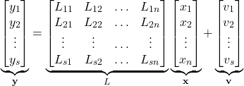
The set of equations in (1) can be compactly written as follows
(3) 
where ![]() and
and ![]() . In (3) and throughout this post, vector quantities are denoted using a bold font. The last equation can be compactly written as follows:
. In (3) and throughout this post, vector quantities are denoted using a bold font. The last equation can be compactly written as follows:
(4) ![]()
In order to formulate the least-squares problem, we need to quantify how accurate is our estimate of scalar variables. Arguably, the most natural way of quantifying the accuracy is to introduce the measurement error
(5) 
Using (4), the last equation can be written compactly as follows
(6) ![]()
where
(7) 
The main idea of the least-squares method is to penalize the weighted sum of squares of the errors. This weighted sum is called a cost function. In the case of the least-squares method, the cost function has the following form
(8) ![]()
where ![]() is defined in (5). In (8), we are dividing the measurement errors by the noise variance. This idea is deeply rooted in engineering intuition and common sense. Namely, if a noise
is defined in (5). In (8), we are dividing the measurement errors by the noise variance. This idea is deeply rooted in engineering intuition and common sense. Namely, if a noise ![]() is significant, then its variance will be large. Consequently, we are less confident that the measurement
is significant, then its variance will be large. Consequently, we are less confident that the measurement ![]() will contain useful information. In other words, we want to put less emphasis on the squared measurement error
will contain useful information. In other words, we want to put less emphasis on the squared measurement error ![]() in the cost function. We can do that by dividing the square of the measurement error by the variance. If the variance has a large value, then the term
in the cost function. We can do that by dividing the square of the measurement error by the variance. If the variance has a large value, then the term ![]() will be relatively small. On the other hand, if the noise in
will be relatively small. On the other hand, if the noise in ![]() is not significant, then the term
is not significant, then the term ![]() will accordingly increase its influence in the overall sum that is represented by
will accordingly increase its influence in the overall sum that is represented by ![]() .
.
From (6)-(7), it follows that the the cost function (8) can be written as
(9) ![]()
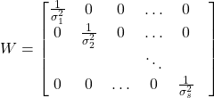
where ![]() is a diagonal weighting matrix defined as follows
is a diagonal weighting matrix defined as follows
(10) 
The least-squares problem can be formally represented as follows:
(11) ![]()
In order to find the minimum of this cost function, we need to compute its gradient and set it to zero. By solving this equation, which is often referred to as the normal equation, we can find an optimal value of ![]() . To compute the gradient, we use the denominator layout notation. In this notation, the gradient is a column vector, and more background information about this notation can be found on its Wikipedia page. To find the gradient of the cost function we use two rules that are outlined in equations (69) and (81) in “The Matrix Cookbook” (2012 version). First, let us expand the expression for
. To compute the gradient, we use the denominator layout notation. In this notation, the gradient is a column vector, and more background information about this notation can be found on its Wikipedia page. To find the gradient of the cost function we use two rules that are outlined in equations (69) and (81) in “The Matrix Cookbook” (2012 version). First, let us expand the expression for ![]() in (9). We have
in (9). We have
(12) ![]()
Next, we need to compute the gradient of ![]() , that is denoted by
, that is denoted by ![]() . Since the gradient is a linear operator (gradient of a sum of elements is equal to the sum of gradients of elements), we need to compute the gradients of every term in (12). The gradients of the following two terms are computed using the equation (69) in “The Matrix Cookbook” (2012 version):
. Since the gradient is a linear operator (gradient of a sum of elements is equal to the sum of gradients of elements), we need to compute the gradients of every term in (12). The gradients of the following two terms are computed using the equation (69) in “The Matrix Cookbook” (2012 version):
(13) 
where we have used the fact that the matrix
(14) ![]()
Finally, using (13) and (14), we can express the gradient of ![]() as follows:
as follows:
(15) ![]()
By setting the gradient to zero, we obtain the system of normal equations:
(16) ![]()
Under the assumption that the matrix ![]() is invertible, we obtain the solution of the least-squares problem
is invertible, we obtain the solution of the least-squares problem
(17) ![]()
where ![]() denotes the matrix inverse of
denotes the matrix inverse of ![]() , and the “hat” notation above
, and the “hat” notation above ![]() is used to denote the solution of the least-squares problem.
is used to denote the solution of the least-squares problem.
In our next post, we are going to explain how to implement the least-squares method in Python and C++.