Dynamics Lecture: Simple Pendulum – Equations of Motion and Solution of Ordinary Differential Equations Using MATLAB – Fusion of Engineering, Control, Coding, Machine Learning, and Science

In this lecture, you will learn to sketch free-body and kinetic diagrams of a simple pendulum. Furthermore, you will learn to develop the equation of motion describing the dynamics of the pendulum. Finally, you will learn how to develop a MATLAB code that solved the equations of motion. A YouTube video accompanying this post is given below.

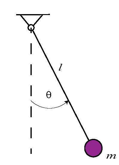
Figure 1 below shows a sketch of a simple pendulum. A simple pendulum consists of a bob of a mass $m$ attached to a cord of length $l$ that can freely oscillate in the gravitational field. The simple pendulum is a simplified model of a number of real-life systems. More about this will be explained in future lectures.

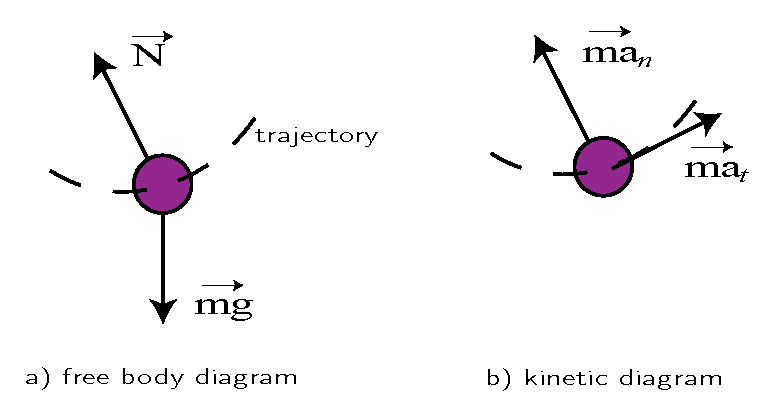
Figure 1: Sketch of a simple pendulum system.

The free-body diagrams and kinetic diagrams of the bob are shown in Fig.2 below (Sketch the free body diagram of the bob by yourself).

From the second Newton law we have:

(1) $\begin{align*}m\vec{a}=\sum_{i=1}^{N} \vec{F}_{i}= m\vec{g}+\vec{N}\end{align*}$

where

(2) $\begin{align*} \vec{a}= \vec{a}_{t}+ \vec{a}_{n} \end{align*}$

Now, the natural coordinate system for projecting the equation (1) is formed by the normal and tangential components of the acceleration vector that are shown in Fig. 2.
By projecting the equation on the tangential unit vector (tangential axis), we obtain

(3) $\begin{align*}ma_{t}=-mg\sin (\theta)\end{align*}$

From the last equation, we obtain:

(4) $\begin{align*}a_{t}+g \sin (\theta) =0\end{align*}$

Since the velocity is given by

(5) $\begin{align*}v=l\dot{\theta}\end{align*}$

The tangential acceleration is given by

(6) $\begin{align*}a_{t}=l\ddot{\theta}\end{align*}$

By substituting the last equation in (5), and by didividing the resulting equation by $l$ , we obtain the final equation of motion:

(7) $\begin{align*}\ddot{\theta}+\frac{g}{l}\sin(\theta) =0\end{align*}$

This is a nonlinear second order differential equation. It is nonlinear since there is a nonlinear function $\sin (\theta)$ in the equation. It is of the second order since, the maximum derivative is of the second order.

To numerically solve this equation using MATLAB, we will transform this equation in the state-space form. First, we need to assign the state-space variables:

(8) $\begin{align*}x_{1}=\theta,\;\; x_{2}=\dot{\theta}\end{align*}$

From the last equation and the equation (7), we have:

(9) $\begin{align*}\dot{x}_{1}=\dot{\theta}=x_{2}\end{align*}$

and

(10) $\begin{align*}\dot{x}_{2}=\ddot{\theta}=- \frac{g}{l}\sin(\theta) = - \frac{g}{l}\sin(x_{1}) \end{align*}$

The equations (9) and (9) can be compactly written as a single vector equation:

(11) $\begin{align*}\begin{bmatrix} \dot{x}_{1} \\ \dot{x}_{2} \end{bmatrix} =\begin{bmatrix} x_{2} \\ -\frac{g}{l}\sin(x_{1}) \end{bmatrix}\end{align*}$

The vector equation (11) is a state-space form of the equation of motion (7). So, we have written the second order differential equation as a system of two first order differential equation. Now, that we have a state-space model of our original equation of motion, we can easly solve it using MATLAB.
The first step is to define the state-space model in a separate MATLAB function. The code is given below.

function dx=dynamics_pendulum(t,x)
mass=1; % define the mass of the bob
l=0.5; % define the length of the cord
g=9.81; % gravitational acceleration

% define the state-space model
dx=[x(2,1); -(g/l)*sin(x(1,1))];
end

The arguments of this function are time $t$ and $2x1$ vector $x$ . The entries of this vector, denoted by x(1,1) and x(2,1) correspond to the state-space variables $x_{1}$ and $x_{2}$ defined above. The state-space model is defined on the code line 7. This code line corresponds to the equation (11). The variable dx corresponds to the right-hand-side of this equation. This function should be saved in the file “dynamics_pendulum.m”, and the folder containing this function should be added to the MATLAB path.
Finally, from the next MATLAB script, we can execute the following code

% time vector 
time_step=0.05
time_vector=[0:time_step:10];
% initial condition 
x0=[0;1]

[time_vector2,solution]=ode45(@dynamics_pendulum,time_vector,x0);


plot(time_vector2,solution(:,1),'r')
grid
hold on
plot(time_vector2,solution(:,2),'k')

The numerical solution approximates the exact solution of the system at the discrete-time steps defined in the vector “time_vector” defined on the line 3. The variable “time_step” defines the discretization time step. In our case, we will approximate the solution from the time instant $0$ seconds until time instant $10$ seconds. The code line 5 defines the initial condition, in our case $x_{1}(0)=0$ and $x_{2}(0)=1$ . Finally, the code line 7 calls the MATLAB ode45() solver. This is a built-in MATLAB function for solving ordinary differential equations. The first argument of this function tells to ode45() solver the name of the file in which the state-space model is defined. In our case, it is the file “dynamics_pendulum.m”. The symbol @ means “at”. The second argument defines the time vector containing discrete time instant for which the solution will be approximated and the third parameter is the initial condition. The ode45() function returns two variables: “time_vector2” containing time instants (that is in our case equal to “time_vector”) and the solution matrix, represented by the variable “solution”. The first column of this matrix corresponds to the solution $x_{1}$ while the second column corresponds to the solution $x_{2}$ . Finally, on lines 10-13, we plot the solution. The results are given in Figure 3 below.

admin

You might also like

Introduction to Eigen C++ Matrix Library

Introduction to inverse kinematics of robots

Rotation Matrix Tutorial for Robotics and Aerospace Engineering – Z-Axis Rotation Matrix