Control Systems Lecture: Overshoot and Peak Time as Functions of Damping Ratio and Natural Undamped Frequency – Complete Derivation – Fusion of Engineering, Control, Coding, Machine Learning, and Science

In this post and in the accompanying YouTube video tutorial we derive the formulas (functions) for overshoot and peak time. We show that peak time is a function of the damping ratio and natural undamped frequency of a prototype second-order system. On the other hand, we show that the overshoot is only a function of the damping ratio. The significance of these formulas originates from the fact that they are often used during the design of control algorithms. Namely, as an input to control system design, we often specify the desired behavior in the time domain. For example, we want to design a control system whose overshoot will be less than 15 percent and the rise time or a peak time will be less than 0.1 second. The main challenge is how to determine the desired closed-loop pole locations that will achieve this design specification. If we know the closed loop poles, then we can use the pole placement method to design the controller.

To solve this problem, we often use the so-called second-order prototype system that is parametrized by the natural frequency and damping ratio of the system poles. The second-order prototype system can often be a good approximation of higher-order systems. In the sequel, we explain how to derive maybe two of the most important formulas for classical control system design. These formulas relate the time domain specifications, such as overshoot and peak time, with the locations of the poles of the prototype second-order system. The derived formulas are often used in control system design to quickly determine the location of the closed-loop poles based on the time domain specifications. We will explain how these formulas are used for control system design in our future tutorials. For the time being, it is important to understand these formulas, and the best way of understanding them is to learn how to derive them. The derivation of these formulas is the main topic of this tutorial. The YouTube video accompanying this post is given below.

Summary of the derived formulas

The peak time and the overshoot are shown in Fig. 1 below.

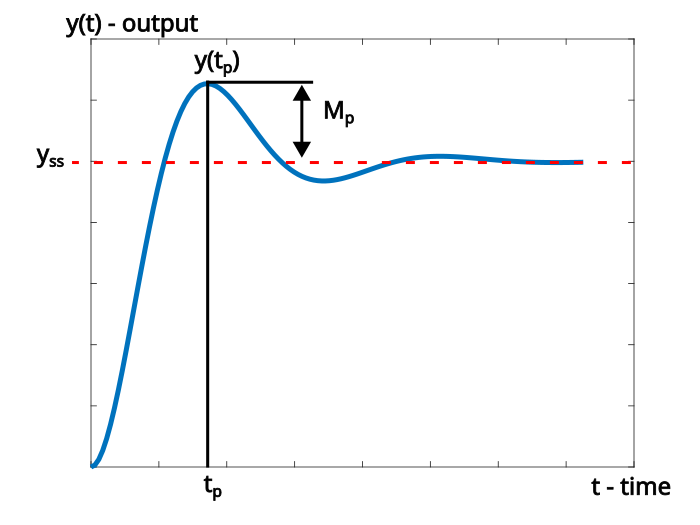
To make the long story short, the peak time is given by

(1) $\begin{align*}t_{p} = \frac{\pi}{\omega_{n} \sqrt{1-\zeta^2}}\end{align*}$

where $\omega_{n}$ is the natural undamped frequency and $\zeta$ is the damping ratio. On the other hand, the overshoot is given by the following formula

(2) $\begin{align*}M_{p}= e^{- \frac{\zeta \pi}{\sqrt{1-\zeta^2}} } \end{align*}$

The percentage overshoot is given by

(3) $\begin{align*}M_{\%p}= e^{- \frac{\zeta \pi}{\sqrt{1-\zeta^2}} } \cdot 100 \%\end{align*}$

From equation (3), we can express the damping ratio as follows

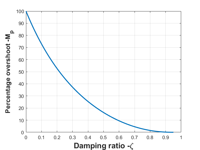
(4) $\begin{align*}\zeta&= \frac{ -\ln (\frac{M_{\% p}}{100})}{\sqrt{\pi^{2} + \ln^{2} (\frac{M_{\% p}}{100})}}\end{align*}$

The following graph is important for the control system design. It is based on (3}), and its shows percentage overshoot as a function of the damping ratio $\zeta$ .

Figure 2: Percentage overshoot as a function of the damping ratio.

The MATLAB code used to generate this figure is given below.

zeta=0:0.01:0.95;

for i=1:numel(zeta)
Mp_percentage(i)= exp(-(zeta(i)*pi)/(sqrt(1-zeta(i)^(2))))*100;
    
end


plot(zeta, Mp_percentage)

Derivation of the formulas for the peak time, overshoot, percentage overshoot, and damping ratio

These formulas are derived under the assumption that our system is of the second order. Moreover, we assume a prototype second-order system given by the following transfer function

The prototype second-order system has the following form:

(5) $\begin{align*}W(s)=\frac{\omega_{n}^{2}}{s^2+2\zeta \omega_{n} s +\omega_{n}^{2}}\end{align*}$

where

$s$ is the complex variable
$\omega_{n}$ is the natural undamped frequency
$\zeta$ is the damping ratio

When deriving the formulas, we assume that the input of the system is a step signal. The output is then

(6) $\begin{align*}Y(s)=W(s)U(s), \;\;\; U(s)=\frac{1}{s}\end{align*}$

In our previous post, which can be found here, we derived an analytical form of the step response in the time domain. The response has the following form

(7) $\begin{align*}y(t)& =1- \frac{e^{-\zeta \omega_{n} t}}{\sqrt{1-\zeta^2}} \sin((\omega_{n} \sqrt{1-\zeta^2}) t +\cos^{-1}(\zeta))\end{align*}$

With this formula, it is always a good idea to specify the following figure (see below) that illustrates the poles of the prototype system (5). A detailed explanation of this figure can be found in our previous post that can be found here.

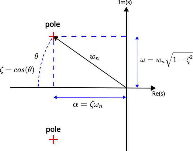
Figure 3: Illustration of the poles of the prototype transfer function (5).

For the derivations that will be presented in the sequel, let us simplify the notation in the expression (7), by introducing the following constants (that are explained in Fig. 3):

(8) $\begin{align*}\alpha & = \zeta \omega_{n} \\\omega & = \omega_{n} \sqrt{1-\zeta^2}\end{align*}$

By using this new notation, we can simplify the formula as follows

(9) $\begin{align*}y(t)& =1- \frac{e^{-\alpha t}}{\sqrt{1-\zeta^2}} \sin(\omega t +\cos^{-1}(\zeta))\end{align*}$

We use the following trigonometric formula, to expand the expression (9):

(10) $\begin{align*}\sin(\gamma+\delta)=\sin(\gamma)\cos(\delta)+\cos(\gamma)\sin(\delta)\end{align*}$

By using this formula in (9), we obtain

(11) $\begin{align*}y(t)=1-\frac{e^{-\alpha t}}{\sqrt{1-\zeta^2}}(\sin(\omega t)\cos(\cos^{-1}(\zeta))+\cos(\omega t) \sin(\cos^{-1}(\zeta))) \end{align*}$

We can simplify the previous expression, by using the following identity:

(12) $\begin{align*}\cos(\cos^{-1}(\zeta))=\zeta \\\end{align*}$

and the following identity that follows from Fig. 1.

(13) $\begin{align*}\sin(\cos^{-1}(\zeta))=\sin(\theta)=\frac{\omega_{n}\sqrt{1-\zeta^2}}{\omega_{n}}=\sqrt{1-\zeta^2}\end{align*}$

By using these expressions in (13), we obtain

(14) $\begin{align*}y(t)& =1-\frac{e^{-\alpha t}}{\sqrt{1-\zeta^2}}(\zeta \sin(\omega t)+\sqrt{1-\zeta^2}\cos(\omega t) ) \\y(t)& =1-e^{-\alpha t}(\frac{\zeta}{\sqrt{1-\zeta^2}} \sin(\omega t)+\cos(\omega t) ) \\y(t)& =1-e^{-\alpha t}(\frac{\omega_{n}\zeta}{\omega_{n}\sqrt{1-\zeta^2}} \sin(\omega t)+\cos(\omega t) ) \\y(t)& =1-e^{-\alpha t}(\frac{\alpha}{\omega} \sin(\omega t)+\cos(\omega t) ) \end{align*}$

where in the last equation, we used (8).

To compute the peak time and the overshoot value, we need to find the maximum of the function $y(t)$ defined in the last equation of (14). We find the function maximum by computing the first derivative and setting it to zero. Let us first compute the first derivative:

(15) $\begin{align*}\dot{y}(t) & =\alpha e^{-\alpha t} (\frac{\alpha}{\omega} \sin(\omega t)+\cos(\omega t)) \\& -e^{-\alpha t}(\frac{\alpha}{\omega} \omega \cos(\omega t)- \omega \sin(\omega t)) \\\dot{y}(t) & = e^{-\alpha t} (\frac{\alpha^2}{\omega}\sin(\omega t)+\omega \sin(\omega t )) \\\dot{y}(t) & =e^{-\alpha t} (\frac{\alpha^2}{\omega}+\omega)\sin(\omega t)\end{align*}$

The extremum points are obtained for time instants for which $\dot{y}(t)=0$ , that is for

(16) $\begin{align*}\sin(\omega t) =0\\ \omega t= k \pi , \;\; k=0,1,2,\ldots\end{align*}$

The first maximum (peak of the transient response) is obtained for $k=1$ :

(17) $\begin{align*}t_{p} = \frac{\pi}{\omega}=\frac{\pi}{\omega_{n} \sqrt{1-\zeta^2}}\end{align*}$

This is our peak time. To find the peak value of the response and the overshoot, we substitute (17) in (15), while keeping in mind the expressions given by (16). The peak value is given by

(18) $\begin{align*} y(t_{p}) & =1- e^{-\alpha t_{p}}(\cos(\omega t_{p})), \\ &\cos(\omega t_{p}) =-1, \;\; \text{since} \;\; \omega t_{p}=\pi \; => \\ y(t_{p})& =1+e^{-\alpha t_{p}} \\y(t_{p})& =1+e^{- \frac{\zeta \omega_{n} \pi}{\omega_{n} \sqrt{1-\zeta^2}} } \\y(t_{p})& =1+e^{- \frac{\zeta \pi}{\sqrt{1-\zeta^2}} } \end{align*}$

The peak value, denoted by $M_{p}$ , is defined by the following expression

(19) $\begin{align*}M_{p}=y(t_{p})-y_{ss}\end{align*}$

Since the system is stable, by using the final value theorem, we obtain

(20) $\begin{align*}y_{ss}=\lim_{s\rightarrow 0} s \cdot \frac{\omega_{n}^{2}}{s^2+2\zeta \omega_{n} s +\omega_{n}^{2}} \frac{1}{s} =\lim_{s\rightarrow 0} \frac{\omega_{n}^{2}}{s^2+2\zeta \omega_{n} s +\omega_{n}^{2}} = 1\end{align*}$

From this expression, we obtain the overshoot value

(21) $\begin{align*}M_{p}= e^{- \frac{\zeta \pi}{\sqrt{1-\zeta^2}} } \end{align*}$

The percentage overshoot, denoted by $M_{\% p}$ , is defined by

(22) $\begin{align*}M_{\% p}=\frac{M_{p}}{y_{ss}} \times 100 \%\end{align*}$

where $y_{ss}$ is the steady state of the step response. The steady-state step response for the system defined by the transfer function (5) is equal to one. That is, $y_{ss}=1$ . This implies that the percentage overshoot is given by the following equation

(23) $\begin{align*}M_{\% p}= e^{- \frac{\zeta \pi}{\sqrt{1-\zeta^2}} } \times 100 \%\end{align*}$

From (23), we can express the damping ratio as a function of the percentage overshoot as follows:

(24) $\begin{align*}\frac{M_{\% p}}{100}& =e^{- \frac{\zeta \pi}{\sqrt{1-\zeta^2}} } \\\ln (\frac{M_{\% p}}{100}) & = - \frac{\zeta \pi}{\sqrt{1-\zeta^2}} \\\ln^{2} (\frac{M_{\% p}}{100}) & = \frac{\zeta^{2} \pi^{2}}{1-\zeta^2} \\(1-\zeta^2)\ln^{2} (\frac{M_{\% p}}{100}) & = \zeta^{2} \pi^{2} \\\ln^{2} (\frac{M_{\% p}}{100}) & = \zeta^{2} ( \pi^{2} + \ln^{2} (\frac{M_{\% p}}{100})) \\\zeta^{2}&= \frac{\ln^{2} (\frac{M_{\% p}}{100})}{\pi^{2} + \ln^{2} (\frac{M_{\% p}}{100})} \\ \zeta&= \frac{|\ln (\frac{M_{\% p}}{100})|}{\sqrt{\pi^{2} + \ln^{2} (\frac{M_{\% p}}{100})}} \\\zeta&= \frac{ -\ln (\frac{M_{\% p}}{100})}{\sqrt{\pi^{2} + \ln^{2} (\frac{M_{\% p}}{100})}}\end{align*}$

Where in the last equation, we used the fact that

(25) $\begin{align*}|\ln (\frac{M_{\% p}}{100})|=-\ln (\frac{M_{\% p}}{100})\end{align*}$

since $\ln (\frac{M_{\% p}}{100})$ is a negative number according to the second equation in (24). To summarize, the damping ratio as a function of the percentage overshoot is given by the following equation

(26) $\begin{align*}\zeta&= \frac{ -\ln (\frac{M_{\% p}}{100})}{\sqrt{\pi^{2} + \ln^{2} (\frac{M_{\% p}}{100})}}\end{align*}$

Numerical verification of the formulas

We numerically verify the derived formulas for the system defined by the following MATLAB code

zeta=0.4
wn=2
transferFunction= tf([wn^2],[1 2*zeta*wn wn^2])
 
[y,time1]=step(transferFunction)
 
plot(time1,y)

The simulated step response is given in the following graph.

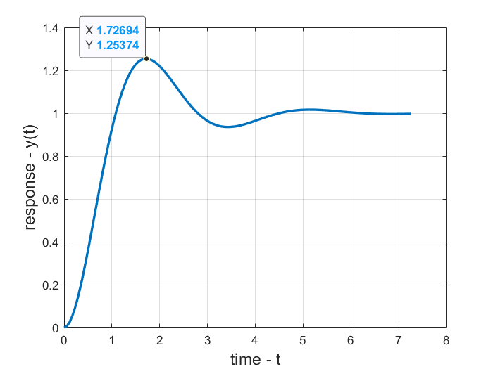
From the graph we obtain $t_{p}\approx 1.25$ and $M_{p}\approx 1.73$ . The system is defined for the following parameters:

(27) $\begin{align*}\zeta=0.4 \\\omega_{n}=2\end{align*}$

For these parameters, from (1):

(28) $\begin{align*}t_{p}=1.7139\end{align*}$

and from (2)

(29) $\begin{align*}M_{p}=0.2538\end{align*}$

Which gives the maximum of the step response equal to $1+M_{p}=1+0.2538=1.2538$ . We can observe that our analytical formulas can accurately predict numerical results.

Summary of the derived formulas

Derivation of the formulas for the peak time, overshoot, percentage overshoot, and damping ratio

Numerical verification of the formulas

admin

You might also like

Introduction to Method of Least Squares

Application of Routh Stability Criterion to Select Parameters of Proportional Integral (PI) Controllers

Setting up Raspberry Pi for Mechatronics Projects – 1