Phase Lead Compensator – Derivation of Equations and Design Procedure – Fusion of Engineering, Control, Coding, Machine Learning, and Science

In this tutorial, we explain the lead controller. We derive the main equations that can be used to design the phase lead controller. In the next post, which can be found here, we present an example of designing the phase lead compensator by using the derived equations. The YouTube tutorial accompanying this tutorial is given below.

Effects of the Phase Lead Compensator

Generally speaking, the phrase lead controller has the following effects on the system performance

The phase margin of the open-loop transfer function is increased. This increases the damping ratio of the closed-loop system and decreases the overshoot of the step response. The rise time is also reduced.
The bandwidth of the closed-loop system is increased.
The slope of the magnitude of the open-loop transfer function is reduced near the crossover frequency. This improves relative system stability.
The steady-state error of the system transient response is not changed.

To illustrate the effect of the phase lead compensator, figures below compare the step responses of the closed loop systems obtained on the basis of the uncompensated and compensated open-loop systems by using the phase lead compensators. The considered open-loop system is:

(1) $\begin{align*}W(s)=\frac{10}{s(s+1)}\end{align*}$

And the compensated open-loop system is

(2) $\begin{align*}W_{c}(s)=\underbrace{\frac{0.4766 s + 1}{0.1036 s + 1}}_{\text{compensator}}\cdot \frac{10}{s(s+1)}\end{align*}$

Fig 1: Close-loop step response of the uncompensated open-loop system (1).

Fig 2: Close-loop step response of the compensated open-loop system (2).

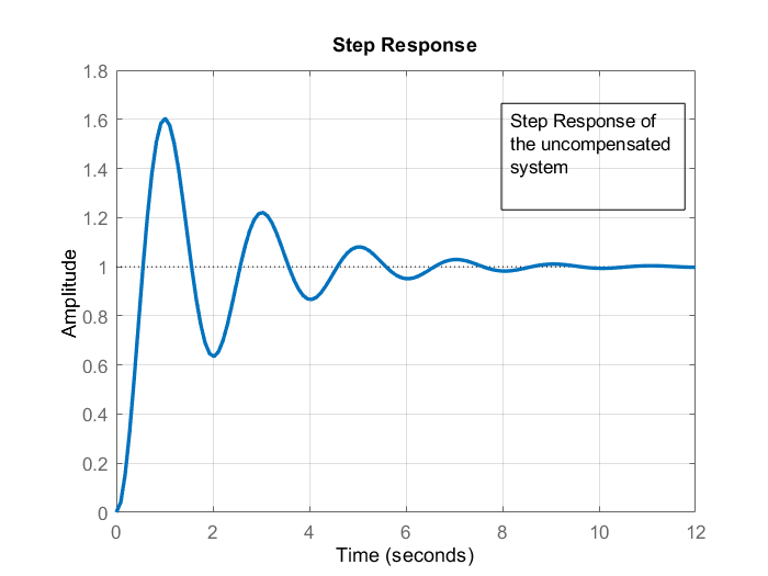
We can observe that the compensator achieves reduced damping and smaller settling time.

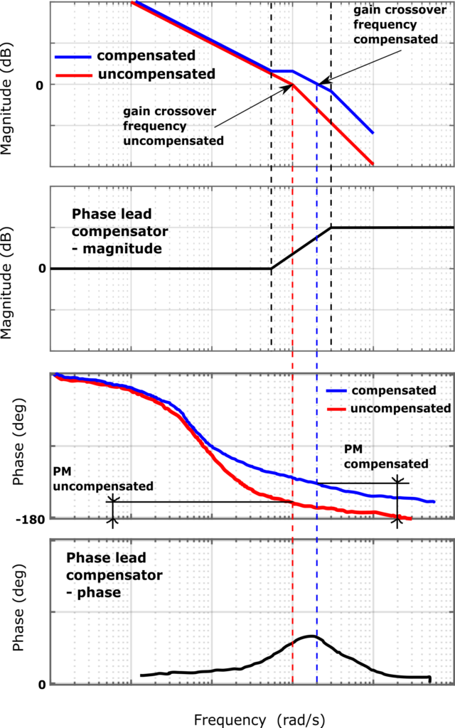
The figure below graphically shows the effect of adding the phase lead controller to the uncompensated system.

Figure 3: The main idea of the phase lead compensator.

Main Equations and Derivations

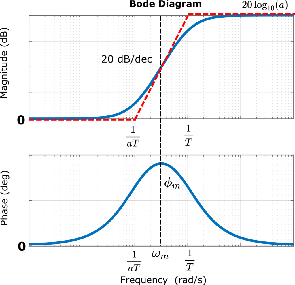
The phase lead compensator is described by the following equation

(3) $\begin{align*}G_{c}(s)=\frac{1+aTs}{1+Ts}\end{align*}$

where $a>1$ and $T>0$ are parameters that need to be designed such that desired behavior is achieved. We can immediately notice that this compensator has two corner frequencies

(4) $\begin{align*}\omega_{1}=\frac{1}{T},\;\; \omega_{2}=\frac{1}{aT}\end{align*}$

We have that $\omega_{2}< \omega_{1}$ since $a>1$ . The generic Bode plot of the lead compensator is shown in the figure below.

Figure 4: Bode plot of the phase lead compensator (23).

The phase lead compensators are usually used to increase the phase margin of the open loop system near the crossover frequency. On the basis of the open loop response of the system, we can evaluate the phase margin. Then, on the basis of the desired phase margin specification, we can determine how much this phase margin needs to be increased. The desired increase of the phase margin is an input parameter for the design of our phase lead compensator. On the basis of the desired change, we need to determine the parameters $a$ and $T$ of the phase lead compensators.

Usually, this is done through the maximum phase of the lead compensator that is denoted by $\phi_{m}$ in Fig. 4. Namely, the desired increase of the phase margin of the open loop system should be roughly equal to $\phi_{m}$ . Then, for such $\phi_{m}$ , we need to determine $a$ and $T$ .

In the sequel, we will derive several formulas that relate $a$ and $\phi_{m}$ . These formulas are used to design the phase lead compensator.

The phase response of the phase lead compensator is given by the following equation:

(5) $\begin{align*}\phi(\omega) = \arctan(aT\omega)-\arctan(T\omega)\end{align*}$

We need to find the maximum of this function. To find the maximum, we will use the following derivative formula

(6) $\begin{align*}\frac{d}{dx}\arctan(x)=\frac{1}{1+x^{2}}\end{align*}$

Applying this formula to (5), we obtain

(7) $\begin{align*}\frac{d}{d\omega} \phi (\omega) =\frac{aT}{1+a^2T^2\omega^2}-\frac{T}{1+T^2\omega^2}=0\end{align*}$

From the last equation, we obtain

(8) $\begin{align*}\frac{d}{d\omega} \phi (\omega) =\frac{aT+a\omega^2 T^{3}-T-a^2T^3\omega^2}{(1+a^2 T^2 \omega^2)(1+\omega^2 T^2)}=0\end{align*}$

From the last equation, we obtain

(9) $\begin{align*}(a-1)(1-a\omega^2T^2)=0\end{align*}$

Let the solution of the last equation be denoted by $\omega_{m}$ (see Fig. 4 also). Then, from the last equation, we have

(10) $\begin{align*}\omega_{m}=\frac{1}{T\sqrt{a}}\end{align*}$

Another method to determine $\omega_{m}$ is by analyzing Fig. 4

. We can observe that

(11) $\begin{align*}\log_{10}(\omega_{m})=\frac{1}{2}\Big( \log_{10}(\frac{1}{aT} ) + \log_{10}(\frac{1}{T} ) \Big)\end{align*}$

From the last equation, we obtain

(12) $\begin{align*}\omega_{m}=\sqrt{\frac{1}{aT^2}}=\frac{1}{\sqrt{a}T}\end{align*}$

By substituting (10) in (5), we obtain

(13) $\begin{align*}\phi(\omega_{m}) & =\phi_m=\arctan(aT\omega_{m})-\arctan(T\omega_{m}) \\\phi_m & =\arctan(\sqrt{a})-\arctan(\frac{1}{\sqrt{a}})\end{align*}$

Our goal is to express $a$ as a function of $\phi_{m}$ from (13). To do that, we first need to recall basic trigonometric identities. First, we have

(14) $\begin{align*}\sin(x-y)=\sin(x)\cos(y)-\cos(x)\sin(y)\end{align*}$

Then, we have

(15) $\begin{align*}\sin(\arctan(x))=\frac{x}{\sqrt{1+x^2}} \\\cos(\arctan(x))=\frac{1}{\sqrt{1+x^2}}\end{align*}$

Next, from (13), we have

(16) $\begin{align*}& \sin(\phi_m) =\sin\big( \arctan(\sqrt{a})-\arctan(\frac{1}{\sqrt{a}})\big)=\\& = \sin(\arctan(\sqrt{a}))\cos(\arctan(\frac{1}{\sqrt{a}}))-\cos(\arctan(\sqrt{a}))\sin(\arctan(\frac{1}{\sqrt{a}}))\end{align*}$

By substituting the above summarized trigonometric formulas, in (16), we obtain

(17) $\begin{align*}\sin(\phi_m) & =\frac{\sqrt{a}}{\sqrt{1+a}}\frac{1}{\sqrt{1+\frac{1}{a}}}-\frac{1}{\sqrt{1+a}}\frac{\frac{1}{\sqrt{a}}}{\sqrt{1+\frac{1}{a}}} \end{align*}$

From the last equation, we obtain

(18) $\begin{align*}\sin(\phi_m)=\frac{a-1}{a+1}\end{align*}$

By solving the last equation for $a$ , we obtain

(19) $\begin{align*}a=\frac{1+\sin(\phi_m)}{1-\sin(\phi_m)}\end{align*}$

Another useful equation for the design of the phase lead compensator is the equation for the asymptotic gain of the lead compensator. This equation is used to estimate how much gain increase the phase lead will produce, and to properly estimate the gain crossover frequency of the compensated system. That is, this equation can help us to properly design the gain crossover frequency of the compensated system. Taking the limit value of (23), we obtain

(20) $\begin{align*}\lim_{s\rightarrow \infty} G_{c}(s)=\lim_{s\rightarrow \infty} \frac{1+aTs}{1+Ts} =a\end{align*}$

Consequently, the magnitude of the Bode plot asymptotically approaches

(21) $\begin{align*}20\log_{10}(a)\end{align*}$

Consider Fig. 4. again, however, this time, take (21) into account. At the point where the phase reaches the maximum value, we have that the gain is half of the gain (21), that is, the gain at $\omega_{m}$ is approximately

(22) $\begin{align*}\text{gain of the compensator at}\;\omega_{c}=\frac{1}{2}20\log_{10}(a)=10\log_{10}(a)\end{align*}$

This conclusion is very important because of the following. Usually, the design goal is to ensure that the compensated system will have a desired gain margin. This means that at the gain crossover frequency of the compensated system, we should have a desired phase margin. We start from the uncompensated system, and we determine the gain crossover frequency and the gain margin of the uncompensated system. Then, on the basis of this information, and on the basis of the desired phase margin of the compensated system, we can select the maximal phase of the lead compensator. Then, we can use the equation (19), to select the parameter $a$ . Then we need to determine the parameter $T$ . This is done by first selecting the frequency $\omega_{m}$ , and then using (10) to compute $T$ . A “naive” approach to compensator design, is to select the parameter $\omega_{m}$ as the gain-crossover frequency of the uncompensated system. In some way, this is logical since we want to add $\phi_{m}$ to the gain margin of the uncompensated system. However, by looking at the magnitude plot of the compensator in Fig. 4, and taking into account (22), we can conclude that the gain of the compensated system will increase at the original gain crossover frequency of the uncompensated system. That is, the gain crossover frequency of the compensated system will change with respect to the gain crossover frequency of the uncompensated system. This means that we cannot accurately tune the phase margin of the compensated system. To tackle this problem, instead of choosing $\omega_{m}$ to be at the gain crossover frequency of the uncompensated system, we choose $\omega_{m}$ to be at the frequency where the gain of the uncompensated system is exactly $-10\log_{10}(a)$ . This means, that once we add the compensator, at the gain cross-over frequency of the compensated system, we will obtain the desired phase margin.

Summary of the Procedure for Designing the Phase Lead Compensator

Design specification and goal: Achieve the Phase Margin (PM) of the compensated system that is larger or equal to the minimum desired value of the PM. Design the parameters $a$ and $T$ of the lead compensator

(23) $\begin{align*}G_{c}(s)=\frac{1+aTs}{1+Ts},\;\; a>1\end{align*}$

PROCEDURE 1:

Step 1: Plot the Bode plot of the uncompensated system. Read the PM of the uncompensated system. On the basis of the PM of the uncompensated system and on the basis of the minimum desired PM, calculate the necessary value of $\phi_{m}$ (maximum phase of the lead compensator), as the difference between the minimum desired PM and the PM of the uncompensated system. That is, $\phi_{m}$ is the value of phase that needs to be added to the PM of the uncompensated system. Optionally, add a few degrees to this difference.

Step 2: For calculated $\phi_{m}$ , determine the parameter $a$ of the compensator by using the following formula

(24) $\begin{align*}a=\frac{1+\sin(\phi_m)}{1-\sin(\phi_m)}\end{align*}$

Step 3: Select $\omega_{m}$ (frequency of the phase lead compensator that produces the maximum phase $\phi_{m}$ of the compensator) as the frequency where the gain of the uncompensated system is equal to $-10\log_{10}(a)$ . This will ensure that the gain cross-over frequency of the compensated system is approximately at $\omega_{m}$ .

Step 4: Select the parameter $T$ as

(25) $\begin{align*}T=\frac{1}{\omega_{m}\sqrt{a}}\end{align*}$

Step 5: Plot the Bode plot, and check if the design specifications are met. If they are met, then we have designed the filter parameters $a$ and $T$ . If not, increase the previously computed value of $\phi_{m}$ , and repeat the steps 2, 3, 4, and 5.

Figure 6 below, explains the main idea of designing the phase lead compensator.

Effects of the Phase Lead Compensator

Main Equations and Derivations

Summary of the Procedure for Designing the Phase Lead Compensator

admin

You might also like

Ray Tracing with COMSOL – First Part

Lab2: Bernoulli equation Lab

Deep Q Networks (DQN) in Python From Scratch by Using OpenAI Gym and TensorFlow- Reinforcement Learning Tutorial