4. Simple moving averages of stock time-series in Pandas and Python – Fusion of Engineering, Control, Coding, Machine Learning, and Science

In this tutorial, we will learn how to

Download and save stock time-series in Pandas and Python.
Compute a simple moving average of time series by writing a “for” loop.
Compute a simple moving average of time series using Panda’s rolling() function.

The GitHub page with the codes used in this and in previous tutorials can be found here. The video accompanying this post is given below.

Let us first, explain what is a moving average. Let $\{x_{k} \}$ be a time series (the notation $\{ x_{k}\}$ denotes a set of discrete-time samples $x_{0},x_{1},x_{2},\ldots$ of the variable $x_{k}$ ). Then a simple moving average of the time series $\{x_{k} \}$ is defined as follows

(1) $\begin{align*}z_{k}=\frac{1}{p}\sum_{i=0}^{p-1} x_{k-j} =\frac{1}{p} \Big(x_{k}+x_{k-1}+\ldots + x_{k-p+1}\Big)\end{align*}$

where ${z_{k}}$ is a new time series obtained from the time series $\{x_{k}\}$ . The positive integer $p$ is called the moving horizon window or the past window. So basically, at the discrete-time instant $k$ , the simple moving average is computed by averaging the last $p$ samples of $x_{k}$ (including the current sample). The main question is what happens at the time instant $k=0$ , since we usually do not have access to the values of $x_{k}$ for negative $k$ . One approach is to simply initialize the values of $x_{k}$ to be zero for $k<0$ . Another approach is to start the computation at $k=p-1$ .

Let us see now how to compute the simple moving average in Python. First we are going to import all the necessary libraries and we are going to download and save Apple stock data to our local computer.

# -*- coding: utf-8 -*-
"""
Moving average of stock prices 
Author:
    Aleksandar Haber
Date: January 21, 2021
Some parts of this code are inspired by the codes given in 
"Learn Algorithmic Trading: Build and deploy algorithmic trading systems and strategies
using Python and advanced data analysis"

by Sebastien Donadio and Sourav Ghosh
"""
# simple moving average implementation in Python and comparison with Pandas 

# standard imports
import pandas as pd 
import numpy as np
import matplotlib.pyplot as plt
# used to donwload the stock prices
import pandas_datareader as pdr

#necessary for computing averages
import statistics as stats

# define the parameters

moving_average_window=40


# define the dates for downloading the data

startDate= '2016-01-01 '
endDate= '2021-01-01'

# Read about Python pickle file format:  https://www.datacamp.com/community/tutorials/pickle-python-tutorial
fileName = 'downloadedData.pkl'

stock_symbol='AAPL'

# this piece of code either reads the data from the saved file or if the saved file does not exist 
# it downloads the data 

try:
    data=pd.read_pickle(fileName)
    print('Loading the data from the local disk.')
except FileNotFoundError:
    print('The data is not found on the local disk.')
    print('Downloading the data from Yahoo.')
    data = pdr.get_data_yahoo(stock_symbol,start=startDate,end=endDate)
    # save the data to file
    print('Saving the data to the local disk.')
    data.to_pickle(fileName)

A few comments about this code are in order. The code line 27 is used to define the moving horizon window. The code lines 32 and 33 are used to define the start and end dates for downloading the stock data. The code line 38 is used to define the stock symbol. In our case, the stock symbol of Apple is “APPL”. Every company that has a corresponding stock has a unique symbol on the stock market exchange. The code lines 43-52 are used to download the stock data and to save it to the local computer. We use an “exception handling” approach in order to increase the code robustness. Under the “try:” code block, we first try to read the data from the local computer. If this code block throws an exception, then the data does not exist on the local computer and the code block under “except FileNotFoundError:” is executed. This code block downloads the data from the Internet using the Pandas function “get_data_yahoo()”.

The following code lines are used to inspect the data and to isolate the time series of “adjusted close prices” that are denoted by the string “Adj Close”.

# inspect the data
    
data.head()

data['Adj Close'].plot()

# isolate the closing price

closingPrice = data['Adj Close']

# isolate the values
closingPrice.values

The code line 9 is used to define the Pandas time series object “closingPrice” that contains the adjusted closing prices. This object will be used to compute the moving average. We explain this in the sequel. The following code lines are used to manually compute the moving average

# computed moving averages
computedMovingAverages=[]

batch=[]


for price in closingPrice.values:
    batch.append(price)
    # if the number of stored entries is larger than the batch capacity, erase the 
    # first entry
    if len(batch) > moving_average_window:
        del(batch[0])
        
    computedMovingAverages.append(stats.mean(batch))
    
# append the original data frame with the computed moving average
# that is, add a column that will contain the values of the computed moving averages

data=data.assign(Moving_average=pd.Series(computedMovingAverages,index=data.index))

A few comments are in order. The variable “computedMovingAverages” is used to store the computed moving averages, and the variable “batch” is used to store the values of past “moving_average_window” samples of the time series. At the end of the computations, we define another column of the “data” Pandas DataFrame object to store the computed moving averages. The following code lines plot the stock prices and moving averages.

fig1=plt.figure(figsize=(10,8))
ax1=fig1.add_subplot(111,ylabel='Stock price in dollars')
data['Adj Close'].plot(ax=ax1, color='b', lw=3, legend=True)
data['Moving_average'].plot(ax=ax1, color='r', lw=3, legend=True )
plt.savefig('moving_average.png')
plt.show()

The results are given in the figure below.

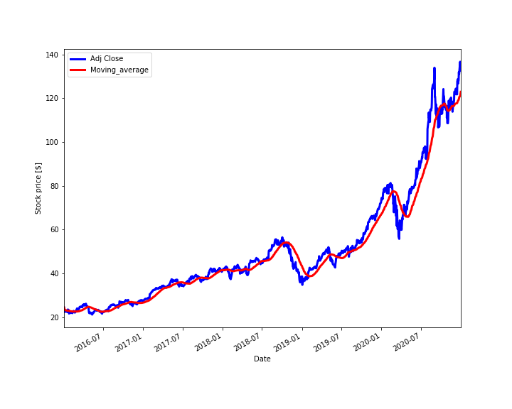
Figure 1: Apple stock prices and computed moving averages.

The blue line in Fig. 1 represents the stock price and the red line represents the computed moving average. Next, it is important that we compare our computations with the built-in Pandas functions for computing the moving averages. The following code lines are used to compute the moving average using the built-in Pandas function “rolling()” and to compare the results with manually computed moving averages. The code is given below.

#check the result using the Pandas rolling() function

moving_average_pandas=data['Adj Close'].rolling(window=moving_average_window).mean()

moving_average_pandas

data['Moving_average']


#compare the results 

fig2=plt.figure(figsize=(10,8))
ax2=fig2.add_subplot(111,ylabel='Moving averages [$]')
data['Moving_average'].plot(ax=ax2, color='r', lw=10, label='Manually computed', legend = True )
moving_average_pandas.plot(ax=ax2, color='k', lw=3, label='Pandas rolling function',  legend = True)
plt.show()

The figure below shows the comparison results.

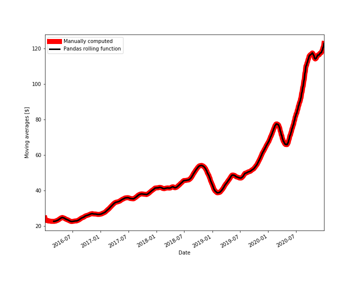
Figure 2: Comparison of the manually computed moving averages with moving averages computed using the Python rolling() function.

From Fig. 2, we can observe that our results match the results produced by the built-in Pandas function, except for the initial 40 values. This is because the Panda’s rolling() function ignores the values of the time series for the time samples that are smaller than the specified moving horizon window.

This is the end of this post. We learned how to compute and plot moving averages of stock prices in Python.

admin

You might also like

Write Numerical or Text Data to File in C Programming Language

Test 4

Pole Placement to Meet the Requirements on Desired Overshoot and Rise Time – Control Engineering Tutorials