5. Accurately Compute Exponential Moving Averages in Pandas and Python – Fusion of Engineering, Control, Coding, Machine Learning, and Science

In our previous post, we have explained how to compute simple moving averages in Pandas and Python. In this post, we explain how to compute exponential moving averages in Pandas and Python. It should be noted that the exponential moving average is also known as an exponentially weighted moving average in finance, statistics, and signal processing communities. The codes that are explained in this post and in our previous posts can be found on the GitHub page. The video accompanying this post is given below.

In order to motivate the definition of the exponential moving averages, let us first consider an average of time series $\{x_{k}\}$ , defined as follows:

(1) $\begin{align*}S_{n}=\frac{x_{n}+x_{n-1}+\ldots + x_{1}}{n}\end{align*}$

where $S_{n}$ is the average and $n$ is the averaging window. The previous equation can be written as follows

(2) $\begin{align*}S_{n}=\frac{n-1}{n}\frac{x_{1}+x_{2}+\ldots + x_{n-1}}{n-1}+ \frac{x_{n}}{n}\end{align*}$

From the last equation, we have

(3) $\begin{align*}S_{n} & =\frac{n-1}{n}S_{n-1}+\frac{x_{n}}{n} \end{align*}$

(4) $\begin{align*}S_{n} & = \Big(1 - \frac{1}{n} \Big)S_{n-1}+\frac{1}{n}x_{n}\end{align*}$

The last equation can be written compactly as follows

(5) $\begin{align*}S_{n} = \Big(1-\beta \Big) S_{n-1}+\beta x_{n}\end{align*}$

(6) $\begin{align*}S_{n} = S_{n-1}+\beta \Big(x_{n}-S_{n-1} \Big)\end{align*}$

where $\beta=\frac{1}{n}$ . The previous derivation is very instructive since as you will see in the sequel, the equation (6) represents a special form of the exponential moving average. Formally speaking, the exponential moving average of the time series $\{x_{k} \}$ is defined by

(7) $\begin{align*}&w_{0}=x_{0} \notag \\ & w_{k}=\alpha x_{k}+ (1-\alpha)w_{k-1}=w_{k-1}+\alpha (x_{k}-w_{k-1}),\;\; \text{for k}>0\end{align*}$

where $\alpha$ is a smoothing factor. Now compare (5) and (6) with (7). We can immediately observe that if $\alpha=\beta=\frac{1}{n}$ , then the exponential moving average becomes the classical average.

Now, the main question is how to select the parameter $\alpha$ . One approach is to try to fit the parameter $\alpha$ from the time series data using optimization methods, for more details, see for example the Wikipedia page.

In the sequel, we are going to use the Pandas ewm() function. From the help page of this function, we see that this function selects the parameter alpha as follows

(8) $\begin{align*}\alpha=\frac{2}{1+s}\end{align*}$

where $s$ is a user-selected time span or a time window. In the sequel, we present the Python code for computing the exponential moving averages. The codes are very similar to the codes that are thoroughly explained in our previous post on simple moving averages and for brevity, we will only provide a brief explanation.

The following code blocks import the necessary libraries, define the parameters, and download and save the stock time series of Apple (the famous company that produces computers, phones, and other electronic devices).

# -*- coding: utf-8 -*-
"""
Exponential moving average of stock prices

https://en.wikipedia.org/wiki/Exponential_smoothing


Author:
    Aleksandar Haber

Date: January 25, 2021
Some parts of this code are inspired by the following sources:
    
-- https://www.datacamp.com/community/tutorials/pickle-python-tutorial
-- Pandas help: https://pandas.pydata.org/pandas-docs/stable/reference/api/pandas.DataFrame.ewm.html
-- "Learn Algorithmic Trading: Build and deploy algorithmic trading systems and strategies
using Python and advanced data analysis", by Sebastien Donadio and Sourav Ghosh
"""


# standard imports
import pandas as pd 
import numpy as np
import matplotlib.pyplot as plt
# used to download the stock prices
import pandas_datareader as pdr

time_period =30 # moving averages window

alpha= 2/(time_period+1) # smoothing factor
# some suggestions for choosing the smoothing factor
# https://pandas.pydata.org/pandas-docs/stable/reference/api/pandas.DataFrame.ewm.html


# define the dates for downloading the data

startDate= '2016-01-01'
endDate= '2021-01-01'

# Read about Python pickle file format:  https://www.datacamp.com/community/tutorials/pickle-python-tutorial
fileName = 'downloadedData.pkl'

stock_symbol='AAPL'

# this piece of code either reads the data from the saved file or if the saved file does not exist 
# it downloads the data 

try:
    data=pd.read_pickle(fileName)
    print('Loading the data from the local disk.')
except FileNotFoundError:
    print('The data is not found on the local disk.')
    print('Downloading the data from Yahoo.')
    data = pdr.get_data_yahoo(stock_symbol,start=startDate,end=endDate)
    # save the data to file
    print('Saving the data to the local disk.')
    data.to_pickle(fileName)

The following code lines are used to inspect and plot the data. We are mainly interested in adjusted closing prices that are denoted by the string “Adj Close” (this is the last column of the “data” object).

# inspect the data

data.head()

data['Adj Close'].plot()

The following code lines are used to compute the exponential moving average of the adjusted closing price and to plot the results.

# isolate the closing price
closingPrice = data['Adj Close']

# isolate the values
closingPrice.values

exponential_moving_average=[] # list used to store the computed exponential moving averages
exponential_moving_average_value=0 # used to store the value of the computed exponential moving average

for price in closingPrice:
    if (exponential_moving_average_value==0): # initialization
        exponential_moving_average_value=price
    else:
        exponential_moving_average_value=alpha*price+(1-alpha)*exponential_moving_average_value
    
    exponential_moving_average.append(exponential_moving_average_value)
    
# append the original data frame with the computed exponential moving average
# that is, add a column that will contain the values of the computed exponential moving averages

data=data.assign(Exponential_moving_average=pd.Series(exponential_moving_average,index=data.index))


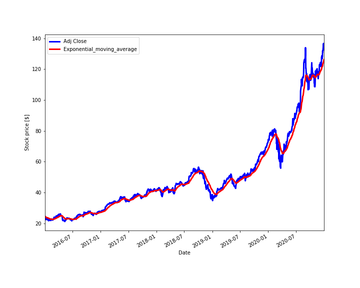
#plot the results

fig1=plt.figure(figsize=(10,8)) 
ax1=fig1.add_subplot(111,ylabel='Stock price in dollars')
data['Adj Close'].plot(ax=ax1, color='b', lw=3, legend=True)
data['Exponential_moving_average'].plot(ax=ax1, color='r', lw=3, legend=True )
plt.savefig('exponential_moving_average.png')
plt.show()

The results are shown in Fig. below.

Figure 1: Computed exponential moving average (red) of the adjusted closing price (blue).

Next, we explain how to easily compute the exponential moving averages using the built-in Pandas function ewm(). We also compare the results with the manually computed exponential moving averages. The code is given below.

# now verify the results by using the Pandas function 
# https://pandas.pydata.org/pandas-docs/stable/reference/api/pandas.DataFrame.ewm.html
exponential_moving_average_pandas=data['Adj Close'].ewm(span=time_period, adjust=False).mean()

# explanation of the parameters
# span :  float, optional - Specify decay in terms of span, α=2/(span+1), for span≥1.
#adjust: bool, default True
# When adjust=False, the exponentially weighted function is calculated recursively:
# y0=x0 
# yt=(1−α)yt−1+αxt,
# CONSEQUENTLY, the parameter "adjust" should be set to "False"

#compare the results 

fig2=plt.figure(figsize=(10,8))
ax2=fig2.add_subplot(111,ylabel='Moving averages [$]')
data['Exponential_moving_average'].plot(ax=ax2, color='r', lw=10, label='Manually computed', legend = True )
exponential_moving_average_pandas.plot(ax=ax2, color='k', lw=3, label='Pandas ewm() function',  legend = True)
plt.savefig('exponential_moving_average_comparison.png')
plt.show()

This code block produces the following figure that compares the Pandas function ewm() with the manual method for computing the exponential moving averages.

Figure 2: Comparison of the Pandas function ewm() with the manual method for computing the exponential moving averages.

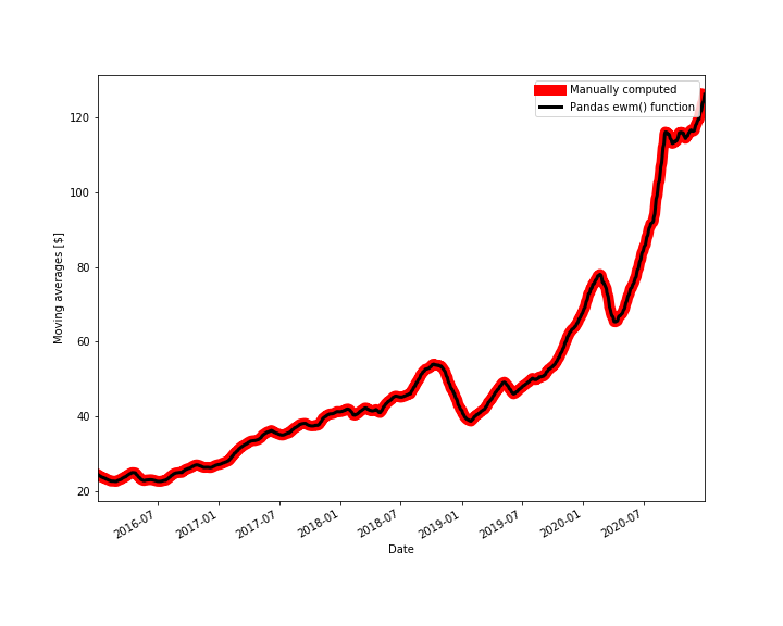
Figure 2 shows that the two methods produce the identical results.

This is the end of this lecture. In this lecture we learned how to compute the exponential moving averages of stock prices using two methods.

admin

You might also like

Easy Explanation of Batch Gradient Descent Method with Python Implementation

Implement Newton’s Method in Python From Scratch by Using SymPy Symbolic Toolbox and Automatic Differentiation

Fourier Series and Frequency Response