 by
by In the video tutorial that is given below, we explain how to compute optical aberrations and Zernike coefficient computations in COMSOL Multiphysics.
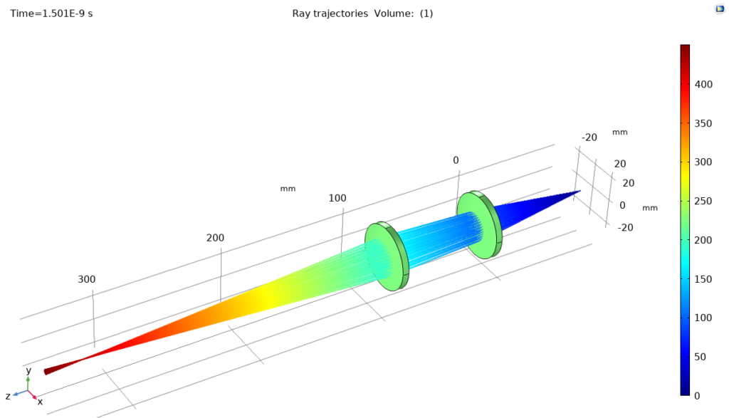
We briefly describe the results. The system consists of two lenses and a point source. For more details, see the video. The ray tracing diagram of the system is shown below.
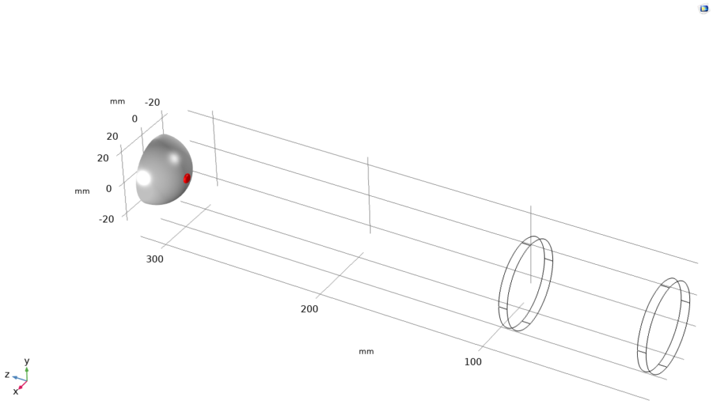
In order to compute the wave-front aberrations in COMSOL, we need to define the reference sphere. The figure below shows the reference sphere for computing the reference sphere. The center of the sphere is placed at the estimated position of the focal plane.
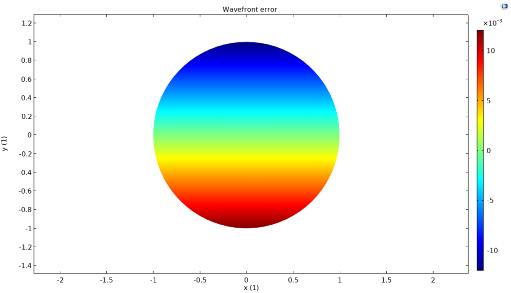
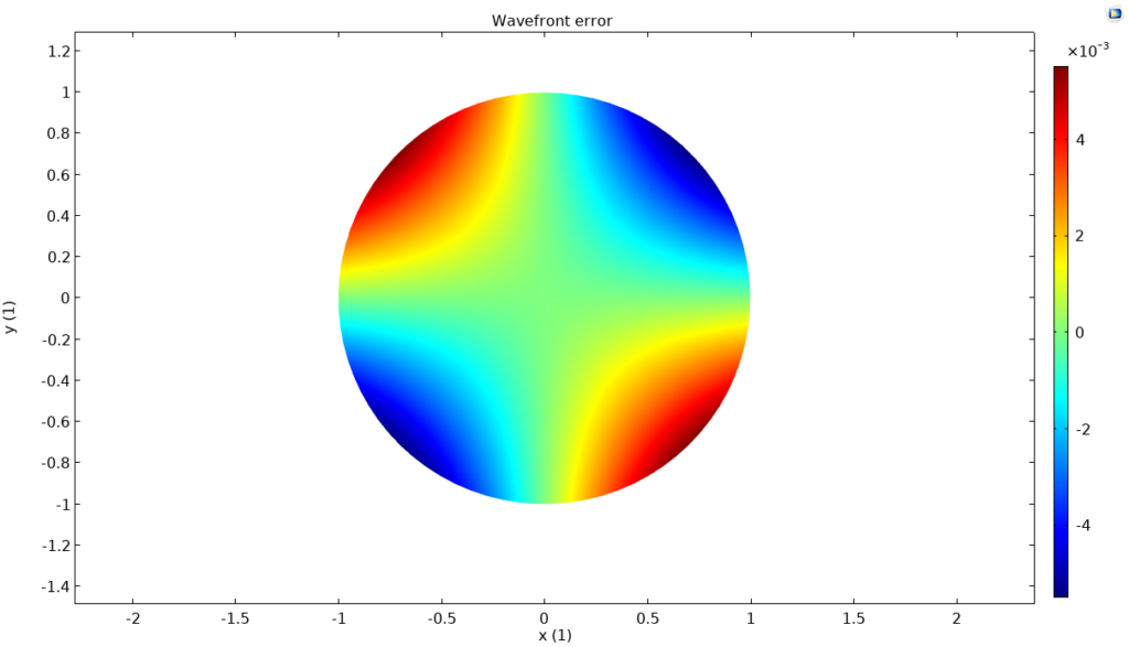
The computer optical aberrations are shown below.
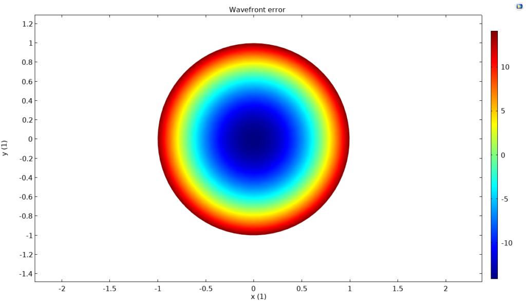
For more details, see the video tutorial.