Bode plot of Second order Transfer Function – Fusion of Engineering, Control, Coding, Machine Learning, and Science

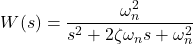
In this tutorial, we explain how to draw a Bode plot of a second order transfer function. We consider a prototype of a second order transfer function

(1) $\begin{align*}W(s)=\frac{\omega_{n}^{2}}{s^{2}+2\zeta \omega_{n} s +\omega_{n}^{2}}\end{align*}$

where

$s$ is the complex Laplace variable
$\omega_{n}$ is the natural undamped frequency
$\zeta$ is the damping ratio

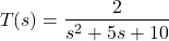
For example, consider the following transfer function

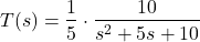
(2) $\begin{align*}T(s)=\frac{2}{s^{2}+5s+10}\end{align*}$

We can write this transfer function as follows

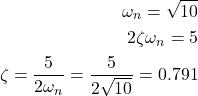
(3) $\begin{align*}T(s)=\frac{1}{5}\cdot \frac{10}{s^{2}+5s+10}\end{align*}$

From this equation, we obtain

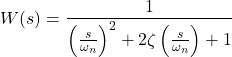
(4) $\begin{align*}\omega_{n}=\sqrt{10} \\2\zeta \omega_{n} = 5 \\\zeta = \frac{5}{2\omega_{n}}= \frac{5}{2 \sqrt{10}} = 0.791\end{align*}$

The first step is to transform the transfer function as follows

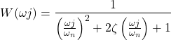
(5) $\begin{align*}W(s)=\frac{1}{\left(\frac{s}{\omega_{n}} \right)^{2}+2\zeta \left( \frac{s}{\omega_{n}} \right) +1}\end{align*}$

Next, we obtain the sinusoidal transfer function, by replacing $s=\omega j$ , where $\omega$ is the angular frequency, and $j=\sqrt{-1}$ :

(6) $\begin{align*}W(\omega j )=\frac{1}{\left(\frac{\omega j }{\omega_{n}} \right)^{2}+2\zeta \left( \frac{\omega j}{\omega_{n}} \right) +1}\end{align*}$

Next, let us recapitulate the polar form of a complex number. For example, consider a complex number

(7) $\begin{align*}z=4+3j\end{align*}$

This complex number can be written in the polar form as

(8) $\begin{align*}z=4+3j= \sqrt{Re^{2} ( z ) + Im^{2} ( z )}\cdot e^{j\cdot \tan^{-1}\left( \frac{Im ( z )}{Re ( z )}\right) }\end{align*}$

(9) $\begin{align*}z=4+3j= \sqrt{4^2 + 3^2}\cdot e^{j \cdot \tan^{-1}\left( \frac{3}{4}\right) } =5 \cdot e^{j\cdot\tan^{-1}\left( \frac{3}{4}\right) }\end{align*}$

To derive the Bode plot, we need to write the sinusoidal transfer function in the polar form, we have

(10) $\begin{align*}W(\omega j )=\frac{1}{1- \left(\frac{\omega }{\omega_{n}} \right)^{2}+2\zeta \left( \frac{\omega }{\omega_{n}} \right)\cdot j}=\frac{1}{D(\omega j)}\end{align*}$

The complex number in the denominator can be written in the polar form

(11) $\begin{align*}D(\omega j)=1- \left(\frac{\omega }{\omega_{n}} \right)^{2}+2\zeta \left( \frac{\omega }{\omega_{n}} \right)\cdot j = \sqrt{\left(1- \left(\frac{\omega }{\omega_{n}} \right)^{2} \right)^{2}+4\zeta^{2} \left( \frac{\omega }{\omega_{n}} \right)^{2} }\cdot e^{j \cdot \tan^{-1} \left(\frac{2\zeta \left( \frac{\omega }{\omega_{n}} \right)}{1- \left(\frac{\omega }{\omega_{n}} \right)^{2}} \right)}\end{align*}$

Consequently, the sinusoidal transfer function can be written as

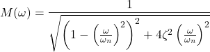
(12) $\begin{align*}W(\omega j)=M(\omega) e^{\phi (\omega) j}\end{align*}$

Where the magnitude function $M(\omega)$ is

(13) $\begin{align*}M(\omega) = \frac{1}{\sqrt{\left(1- \left(\frac{\omega }{\omega_{n}} \right)^{2} \right)^{2}+4\zeta^{2} \left( \frac{\omega }{\omega_{n}} \right)^{2} }}\end{align*}$

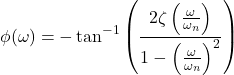
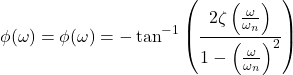
and the phase function is

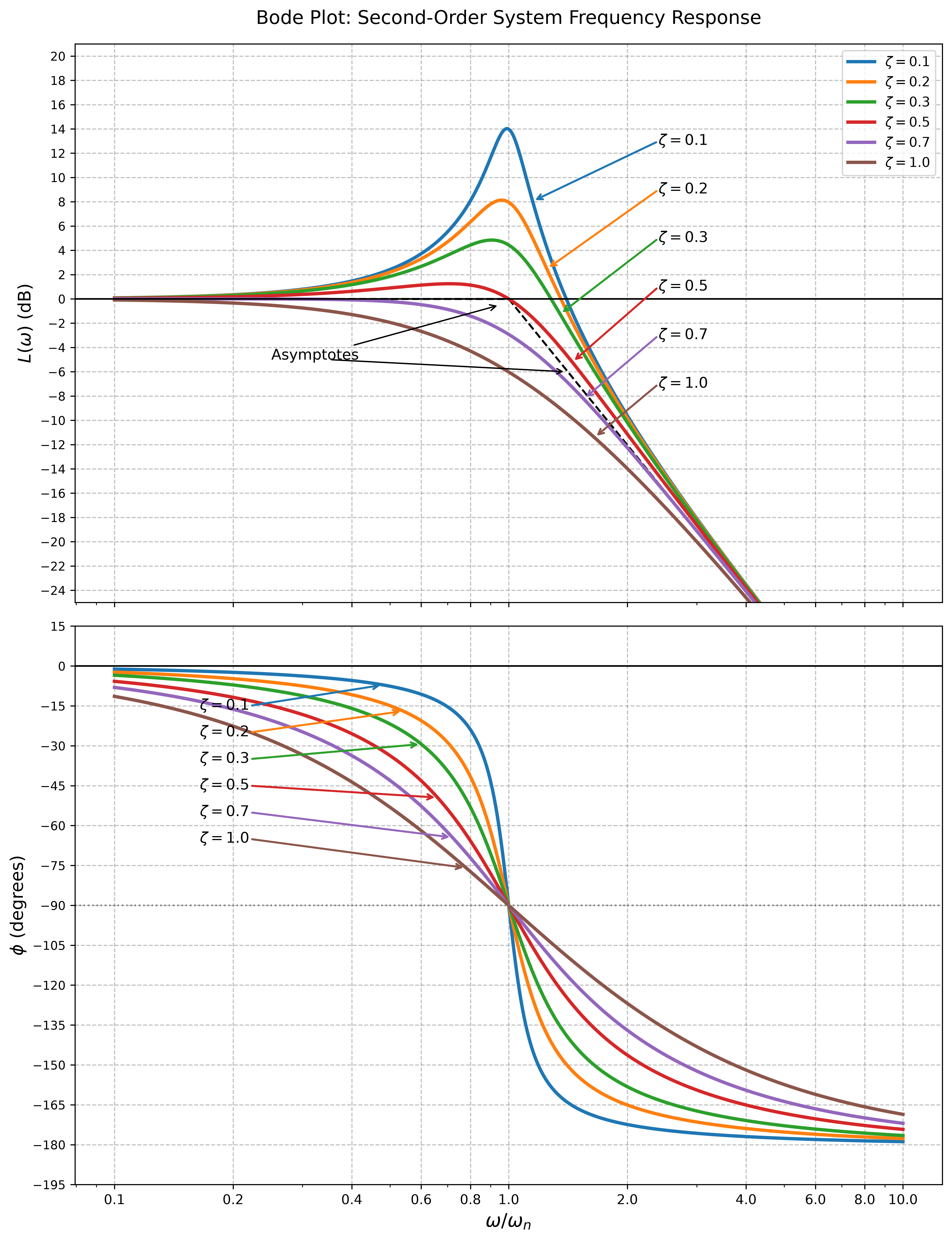
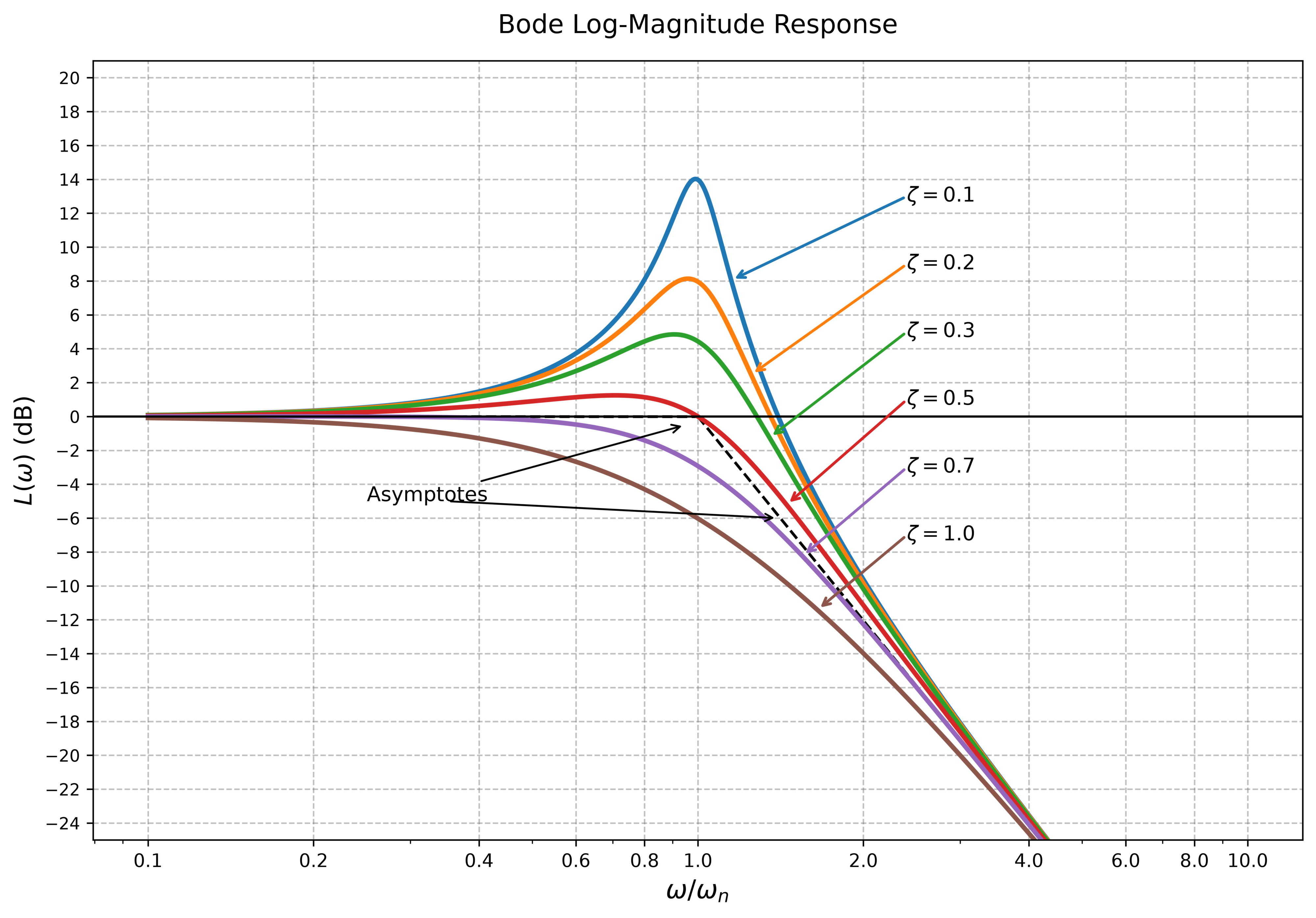
(14) $\begin{align*}\phi (\omega) = - \tan^{-1} \left(\frac{2\zeta \left( \frac{\omega }{\omega_{n}} \right)}{1- \left(\frac{\omega }{\omega_{n}} \right)^{2}} \right)\end{align*}$

The Bode plot consists of the log manitude function

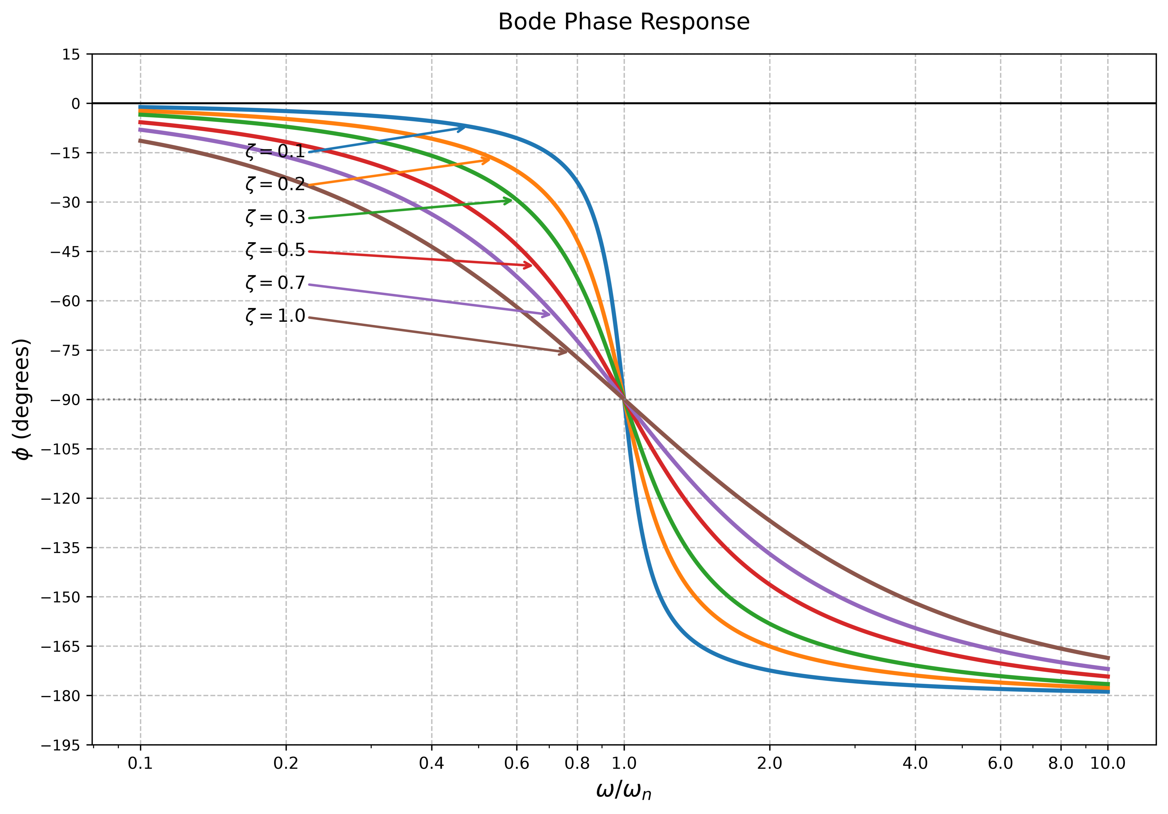
(15) $\begin{align*}L(\omega)=20 \log M(\omega)= - 20 \log \left( \sqrt{\left(1- \left(\frac{\omega }{\omega_{n}} \right)^{2} \right)^{2}+4\zeta^{2} \left( \frac{\omega }{\omega_{n}} \right)^{2} } \right) \end{align*}$

and phase

(16) $\begin{align*}\phi (\omega)= \phi (\omega) = - \tan^{-1} \left(\frac{2\zeta \left( \frac{\omega }{\omega_{n}} \right)}{1- \left(\frac{\omega }{\omega_{n}} \right)^{2}} \right)\end{align*}$

The Bode plot for different values of $\zeta$ and $\omega$ is given below.

The Python code is given below.

import numpy as np
import matplotlib.pyplot as plt
from scipy import signal

# Explicitly maintain the color cycle from the previous plots
colors = ['C0', 'C1', 'C2', 'C3', 'C4', 'C5']
zeta_values = [0.1, 0.2, 0.3, 0.5, 0.7, 1.0]
omega_n = 1.0 

# Frequency range matching the textbook layout (0.1 to 10)
w = np.logspace(-1, 1, 1000)

fig, (ax_mag, ax_phase) = plt.subplots(2, 1, figsize=(9, 11), sharex=True)

# -----------------------------------------------------------------
# 1. Plot Asymptotes
# -----------------------------------------------------------------
w_asymp_low = np.logspace(-1, 0, 100)
w_asymp_high = np.logspace(0, 1, 100)
ax_mag.plot(w_asymp_low, np.zeros_like(w_asymp_low), 'k--', lw=1.5)
ax_mag.plot(w_asymp_high, -40 * np.log10(w_asymp_high / omega_n), 'k--', lw=1.5)

# Asymptote text pointers
ax_mag.annotate('Asymptotes', xy=(0.95, -0.5), xytext=(0.25, -5),
                arrowprops=dict(arrowstyle="->", color="black", lw=1), fontsize=11)
ax_mag.annotate('', xy=(1.4, -6), xytext=(0.35, -5),
                arrowprops=dict(arrowstyle="->", color="black", lw=1))

# -----------------------------------------------------------------
# 2. Compute, Plot, and Precisely Annotate Curves
# -----------------------------------------------------------------
handles = []

# Exact geometric configurations matching the textbook layout
mag_annotation_config = {
    0.1: {'text_pos': (2.4, 13), 'target_w': 1.15},
    0.2: {'text_pos': (2.4, 9),  'target_w': 1.25},
    0.3: {'text_pos': (2.4, 5),  'target_w': 1.35},
    0.5: {'text_pos': (2.4, 1),  'target_w': 1.45},
    0.7: {'text_pos': (2.4, -3), 'target_w': 1.55},
    1.0: {'text_pos': (2.4, -7), 'target_w': 1.65}
}

phase_annotation_config = {
    0.1: {'text_pos': (0.22, -15), 'target_w': 0.48},
    0.2: {'text_pos': (0.22, -25), 'target_w': 0.54},
    0.3: {'text_pos': (0.22, -35), 'target_w': 0.60},
    0.5: {'text_pos': (0.22, -45), 'target_w': 0.66},
    0.7: {'text_pos': (0.22, -55), 'target_w': 0.72},
    1.0: {'text_pos': (0.22, -65), 'target_w': 0.78}
}

for zeta, color in zip(zeta_values, colors):
    num = [omega_n**2]
    den = [1, 2 * zeta * omega_n, omega_n**2]
    sys = signal.TransferFunction(num, den)
    w_out, mag, phase = signal.bode(sys, w)
    
    # Plotting response lines
    line, = ax_mag.plot(w_out, mag, color=color, lw=2.5, label=f'')
    handles.append(line)
    ax_phase.plot(w_out, phase, color=color, lw=2.5)
    
    # --- Magnitude Annotations (Right Side, Pointing Left-Down) ---
    m_cfg = mag_annotation_config[zeta]
    mag_target_y = np.interp(m_cfg['target_w'], w_out, mag)
    
    ax_mag.text(m_cfg['text_pos'][0], m_cfg['text_pos'][1], f'', 
                fontsize=11, va='center', ha='left', color='black')
    ax_mag.annotate('', xy=(m_cfg['target_w'], mag_target_y), xytext=(m_cfg['text_pos'][0], m_cfg['text_pos'][1]),
                    arrowprops=dict(arrowstyle="->", color=color, lw=1.5, connectionstyle="arc3,rad=0"))

    # --- Phase Annotations (Left Side, Pointing Right-Down) ---
    p_cfg = phase_annotation_config[zeta]
    phase_target_y = np.interp(p_cfg['target_w'], w_out, phase)
    
    ax_phase.text(p_cfg['text_pos'][0], p_cfg['text_pos'][1], f'', 
                 fontsize=11, va='center', ha='right', color='black')
    ax_phase.annotate('', xy=(p_cfg['target_w'], phase_target_y), xytext=(p_cfg['text_pos'][0], p_cfg['text_pos'][1]),
                    arrowprops=dict(arrowstyle="->", color=color, lw=1.5, connectionstyle="arc3,rad=0"))

# -----------------------------------------------------------------
# 3. Aesthetics & Axis Formatting
# -----------------------------------------------------------------
for ax in [ax_mag, ax_phase]:
    ax.set_xscale('log')
    ax.grid(True, which='both', linestyle='--', color='gray', alpha=0.5)
    ax.set_xticks([0.1, 0.2, 0.4, 0.6, 0.8, 1, 2, 4, 6, 8, 10])
    ax.get_xaxis().set_major_formatter(plt.ScalarFormatter())

# Upper Subplot formatting
ax_mag.set_ylabel(' (dB)', fontsize=13)
ax_mag.set_ylim(-25, 20)
ax_mag.set_yticks([-20, -10, 0, 10, 20])
ax_mag.axhline(0, color='black', lw=1)
ax_mag.legend(handles=handles, loc='upper right', frameon=True, fontsize=10)
ax_mag.set_title('Bode Plot: Second-Order System Frequency Response', fontsize=14, pad=15)

# Lower Subplot formatting
ax_phase.set_xlabel('', fontsize=14)
ax_phase.set_ylabel(' (degrees)', fontsize=13)
ax_phase.set_ylim(-195, 15)
ax_phase.set_yticks([0, -90, -180])
ax_phase.axhline(0, color='black', lw=1)
ax_phase.axhline(-90, color='gray', linestyle=':', lw=1)

plt.tight_layout()

# Save high-resolution file
plt.savefig("bode_plot_perfect_alignment.png", dpi=600, bbox_inches='tight')
plt.show()

admin

You might also like

COMSOL Tutorial: Thin-Plate Deformation-Introducing Damping

Clear Graphical and Mathematical Explanation of Yaw, Pitch and Roll Euler Angles – Part 2

Simulation of Ordinary Differential Equations (ODEs) with Time-varying Coefficients and Time-varying Inputs in MATLAB