 by
by This is the third post in a series of posts on time series modeling and analysis in Python. In this post, we will learn how to download and analyze financial (stock) time series. We will directly load financial time series data into a Pandas DataFrame structure. Consequently, we will be able to fully exploit the power of Pandas and Python to manipulate the downloaded data. The GitHub page with the codes used in this and in previous tutorials can be found here. The video accompanying this post is given below.
First, we import all the necessary libraries.
import pandas as pd
import numpy as np
import matplotlib.pyplot as plt

import datetime #necessary for creating a datetime object
import pandas_datareader as pdr #necessary for downloading the stock data from Yahoo! Finance
# you need to install this library by opening a command line and by typing "pip install pandas-datareader"
The code lines 1-3 are used to import Pandas, Numpy, and plotting libraries. The code line 5 is used to import a library for defining a “datetime” object. This object is provided as an argument to a function for downloading the financial data. The code line 6 is used to import Pandas “datareader” library that is used to download the financial time series. Before you can import this library you have to install it by opening a command-line editor and by typing: “pip install pandas-datareader”.
The following code lines are used to download the historical stock data of Amazon and Boeing companies.
# load the stock data from internet

start_time=datetime.datetime(2020,1,1)
end_time=datetime.datetime(2021,1,1)

# load the Amazon stock data
amzn=pdr.get_data_yahoo('AMZN', start=start_time, end=end_time)

# load the Boeing stock data
ba=pdr.get_data_yahoo('BA', start=start_time, end=end_time)
The code lines 3 and 4 are used to define the start and end time stamps for obtaining the historical data. The code lines 7 and 10 are used to download the time series and to store them in DataFrame objects “amzn” and “ba”. The previous code lines can be compressed as follows.
# another way for defining the time stamps - using the pd.Timestamp() function

amzn2=pdr.get_data_yahoo('AMZN', pd.Timestamp('2020,01,01'), pd.Timestamp('2021,01,01'))
ba2=pdr.get_data_yahoo('BA', pd.Timestamp('2020,01,01'), pd.Timestamp('2021,01,01'))
We have used “pd.Timestamp(‘.’)” function to provide start and end time stamps.
Next, we explore the downloaded data. By executing the following code line
# investigate the data

amzn.head()
we obtain
                   High          Low  ...   Volume    Adj Close
Date                                  ...
2020-01-02  1898.010010  1864.150024  ...  4029000  1898.010010
2020-01-03  1886.199951  1864.500000  ...  3764400  1874.969971
2020-01-06  1903.689941  1860.000000  ...  4061800  1902.880005
2020-01-07  1913.890015  1892.040039  ...  4044900  1906.859985
2020-01-08  1911.000000  1886.439941  ...  3508000  1891.969971

[5 rows x 6 columns]
The indices can be obtained as follows
# get the index timestamps
amzn.index
DatetimeIndex(['2020-01-02', '2020-01-03', '2020-01-06', '2020-01-07',
               '2020-01-08', '2020-01-09', '2020-01-10', '2020-01-13',
               '2020-01-14', '2020-01-15',
               ...
               '2020-12-17', '2020-12-18', '2020-12-21', '2020-12-22',
               '2020-12-23', '2020-12-24', '2020-12-28', '2020-12-29',
               '2020-12-30', '2020-12-31'],
              dtype='datetime64[ns]', name='Date', length=253, freq=None)
The column names can be obtained by executing
# get the column names
amzn.columns
Index(['High', 'Low', 'Open', 'Close', 'Volume', 'Adj Close'], dtype='object')The stored values can be obtained by executing
amzn_values=amzn.values
array([[1.89801001e+03, 1.86415002e+03, 1.87500000e+03, 1.89801001e+03,
        4.02900000e+06, 1.89801001e+03],
       [1.88619995e+03, 1.86450000e+03, 1.86450000e+03, 1.87496997e+03,
        3.76440000e+06, 1.87496997e+03],
       [1.90368994e+03, 1.86000000e+03, 1.86000000e+03, 1.90288000e+03,
        4.06180000e+06, 1.90288000e+03],
       ...,
       [3.35064990e+03, 3.28121997e+03, 3.30993994e+03, 3.32200000e+03,
        4.87290000e+06, 3.32200000e+03],
       [3.34210010e+03, 3.28246997e+03, 3.34100000e+03, 3.28585010e+03,
        3.20930000e+06, 3.28585010e+03],
       [3.28291992e+03, 3.24119995e+03, 3.27500000e+03, 3.25692993e+03,
        2.95410000e+06, 3.25692993e+03]])
The first three stored (row) values can be accessed as follows
# plot the values at the rows 1,2,3
amzn.values[0:3,:]
array([[1.89801001e+03, 1.86415002e+03, 1.87500000e+03, 1.89801001e+03,
        4.02900000e+06, 1.89801001e+03],
       [1.88619995e+03, 1.86450000e+03, 1.86450000e+03, 1.87496997e+03,
        3.76440000e+06, 1.87496997e+03],
       [1.90368994e+03, 1.86000000e+03, 1.86000000e+03, 1.90288000e+03,
        4.06180000e+06, 1.90288000e+03]])
Basic statistics can be computed by executing
# compute basic statistics
amzn.describe()
High Low ... Volume Adj Close
count 253.000000 253.000000 ... 2.530000e+02 253.000000
mean 2716.941377 2642.261857 ... 4.931556e+06 2680.855096
std 554.291416 539.598841 ... 1.976104e+06 545.761043
min 1759.449951 1626.030029 ... 1.451900e+06 1676.609985
25% 2166.070068 2124.110107 ... 3.476400e+06 2149.870117
50% 2955.560059 2871.000000 ... 4.526600e+06 2890.300049
75% 3202.000000 3130.489990 ... 5.789300e+06 3165.120117
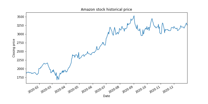
max 3552.250000 3486.689941 ... 1.556730e+07 3531.449951The column “Adj close” represent adjusted closing prices of stocks. The values stored in this column can be plotted as follows.
#plot the closing prices
ax1=amzn['Adj Close'].plot(figsize=(10,5),title='Amazon stock historical price')
ax1.set_xlabel('Date')
ax1.set_ylabel('Closing price')
# save the figure to a file
plt.savefig('amzn.png')
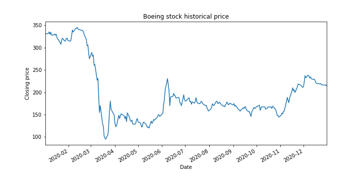
#plot the closing prices
ax2=ba['Adj Close'].plot(figsize=(10,5),title='Boeing stock historical price')
ax2.set_xlabel('Date')
ax2.set_ylabel('Closing price')
# save the figure to a file
plt.savefig('ba2.png')
Once we have downloaded the data, it is a good idea to save the data to a file. The following code lines save the downloaded time series to a file, load the saved data into a new variable, and plot the time series.
# save data to a file
amzn.to_csv('amzn_data.csv')

# load data from the saved file
loaded_amzn=pd.read_csv('amzn_data.csv')

loaded_amzn['Adj Close'].plot(figsize=(10,5))
The monthly means can be computed as follows
# resample the data
monthly_resampled_amzn=amzn['Adj Close'].resample('M').mean()

monthly_resampled_amzn

monthly_resampled_amzn.plot()
The difference between the open and closing prices can be computed as follows
# add a new column to data that is difference


amzn['diff']=amzn['Open']-amzn['Close']

amzn.columns
amzn.head()
amzn['diff'].plot()
Notice that we have added a new column to the DataFrame structure that represents the computed difference. This column can be erased as follows
# delete a column

del amzn['diff']

amzn.columns
The adjusted closing prices of Amazon and Boeing stocks can be concatenated as follows
#concatenate

#concatenate

close_amzn=amzn['Adj Close']
close_ba=ba['Adj Close']

close_concat=pd.concat([close_amzn,close_ba],axis=1)

close_concat.head()

close_concat.columns
              Adj Close   Adj Close
Date
2020-01-02  1898.010010  331.348572
2020-01-03  1874.969971  330.791901
2020-01-06  1902.880005  331.766083
2020-01-07  1906.859985  335.285156
2020-01-08  1891.969971  329.410095

Index(['Adj Close', 'Adj Close'], dtype='object')
Two DataFrames can also be concatenated. This can be achieved by executing the following code lines
# concatenate everything

concat=pd.concat([amzn,ba], axis=1)

concat.head()

concat.columns
                   High          Low  ...     Volume   Adj Close
Date                                  ...
2020-01-02  1898.010010  1864.150024  ...  4544400.0  331.348572
2020-01-03  1886.199951  1864.500000  ...  3875900.0  330.791901
2020-01-06  1903.689941  1860.000000  ...  5355000.0  331.766083
2020-01-07  1913.890015  1892.040039  ...  9898600.0  335.285156
2020-01-08  1911.000000  1886.439941  ...  8239200.0  329.410095

Index(['High', 'Low', 'Open', 'Close', 'Volume', 'Adj Close', 'High', 'Low',
       'Open', 'Close', 'Volume', 'Adj Close'],
      dtype='object')
The data can be concatenated in a more elegant way. This can be achieved by assigning the keys, so we can easily retrieve the data.
# acessing the entries
concat2.head()

concat2['AMZN'].head()

concat2['AMZN']['Adj Close'].head()

concat2['AMZN']['Adj Close'].loc['2020-01-02']
                   AMZN               ...         BA
                   High          Low  ...     Volume   Adj Close
Date                                  ...
2020-01-02  1898.010010  1864.150024  ...  4544400.0  331.348572
2020-01-03  1886.199951  1864.500000  ...  3875900.0  330.791901
2020-01-06  1903.689941  1860.000000  ...  5355000.0  331.766083
2020-01-07  1913.890015  1892.040039  ...  9898600.0  335.285156
2020-01-08  1911.000000  1886.439941  ...  8239200.0  329.410095


                   High          Low  ...   Volume    Adj Close
Date                                  ...
2020-01-02  1898.010010  1864.150024  ...  4029000  1898.010010
2020-01-03  1886.199951  1864.500000  ...  3764400  1874.969971
2020-01-06  1903.689941  1860.000000  ...  4061800  1902.880005
2020-01-07  1913.890015  1892.040039  ...  4044900  1906.859985
2020-01-08  1911.000000  1886.439941  ...  3508000  1891.969971


concat2Date
2020-01-02    1898.010010
2020-01-03    1874.969971
2020-01-06    1902.880005
2020-01-07    1906.859985
2020-01-08    1891.969971
Name: Adj Close, dtype: float64


1898.010009765625