Phase Portraits of State-Space Models and Differential Equations in Python – Fusion of Engineering, Control, Coding, Machine Learning, and Science

In this post, we explain

The basics of phase portraits of dynamical systems and state-space models.
How to plot phase portraits in Python

A YouTube video accompanying this tutorial is given below.

The GitHub page with the codes presented in this tutorial is given here. Besides this tutorial, we created a tutorial on how to generate phase portraits of dynamical systems in MATLAB. The MATLAB tutorial is given here.

Basics of Phase Portraits of Dynamical Systems

For example, consider the following dynamical system:

(1) $\begin{align*}\dot{\mathbf{x}}=\begin{bmatrix}-x_{1}-3x_{2} \\ 3x_{1} -x_{2}\end{bmatrix}\end{align*}$

This is a state-space model a dynamical system with two state-space variables $x_{1}$ and $x_{2}$ . In this tutorial, you will learn how to generate a phase portrait of this system in Python. The phase portrait is shown in the figure below.

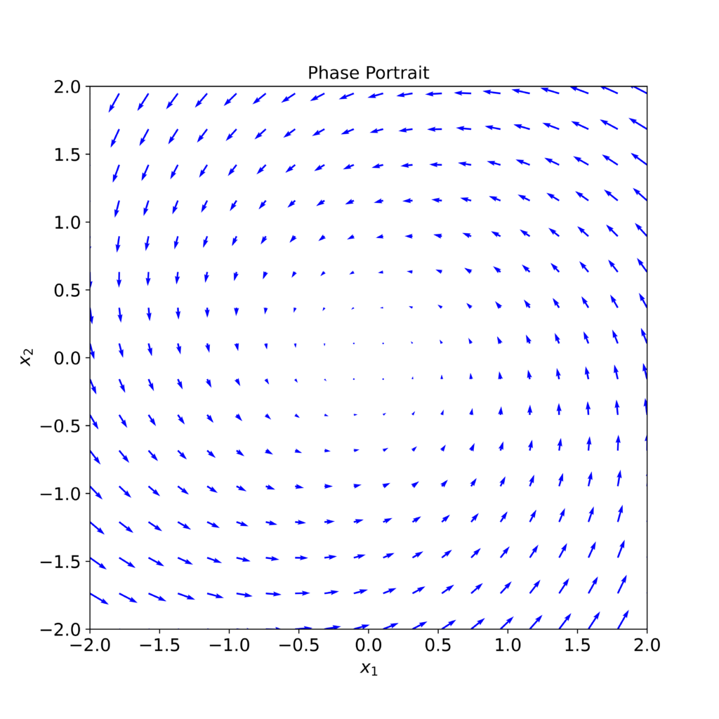
Figure 1: Phase portrait of the system given by the equation (1).

An arrow at a certain point is actually a tangent to the state-space trajectory at that point. Loosely speaking, during the small time interval, the direction of the arrow denotes the direction of the state-space trajectory evolution at a particular point.

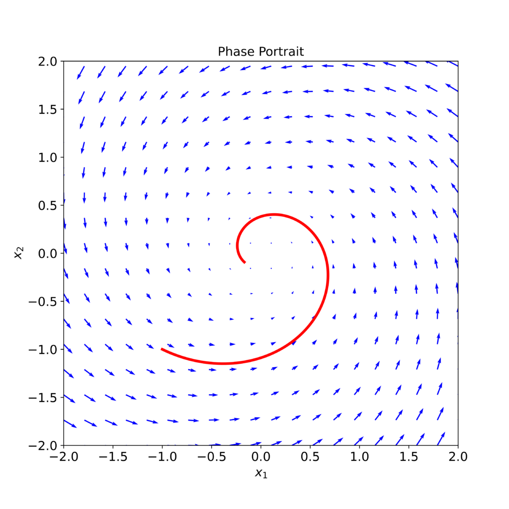
Besides learning how to plot a phase portrait of a dynamical system, you will learn how to plot a particular state-space trajectory obtained by simulating (1) from a given initial state. A simulated state trajectory (red line) is shown in Figure 2 below. This state-space trajectory is generated for the initial conditions $x_{1}=-1$ and $x_{2}=-1$ .

Figure 2: State-space trajectory starting from the initial condition $(x_{1}=-1,x_{2}=-1)$ .

Figure 2: State-space trajectory starting from the initial condition $(x_{1}=-1,x_{2}=-1)$ .

Let us now explain the main idea for constructing phase portraits. Consider the general form of a state-space model of a dynamical system:

(2) $\begin{align*}\dot{\mathbf{x}}=\begin{bmatrix} f_{1}(x_{1},x_{2}) \\ f_{2}(x_{1},x_{2}) \end{bmatrix}\end{align*}$

The vector $\dot{\mathbf{x}}$ defines a tangent to the state-space trajectory. This tangent is shown in Fig. 3 below.

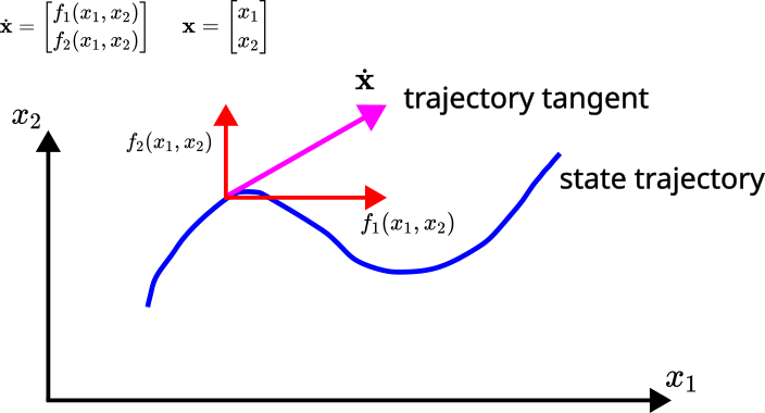
Figure 3: Tangent to the state-space trajectory with its projections.

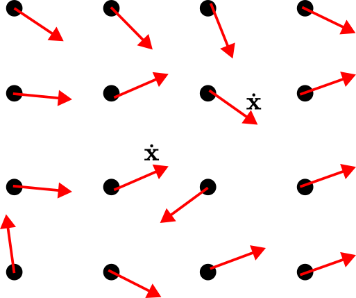
The components of the tangent vector $\dot{\mathbf{x}}$ are $f_{1}(x_{1},x_{2})$ and $f_{2}(x_{1},x_{2})$ . Consequently, for known values of $x_{1}$ and $x_{2}$ we can construct the tangent vector $\dot{\mathbf{x}}$ . The tangent vectors at trajectory points define the phase portraits. Consequently, to construct the phase portrait, we construct a grid of state-space points shown in Fig. 4. Then, at every point of this grid, we calculate the $x_{1}$ and $x_{2}$ projections of the tangent vector and construct the tangent vector. These tangent vectors define the phase portrait.

Figure 4: Grid of state-space points for constructing the phase portraits. At every point of this grid, we can construct a tangent vector to the state-space trajectory.

Python Code for Generating Phase Portraits

The first step is to import the necessary libraries and functions and to define a function that corresponds to the right-hand side of our state-space model. The code is given below.


import matplotlib.pyplot as plt
from scipy.integrate import odeint
import numpy as np

# first create create a function that evaluates the right-hand-side of the
# state-space equations for a given state vector

# x is the current state vector 
# t is current simulation time

def dynamicsStateSpace(x,t):
    dxdt=[-x[0]-3*x[1],3*x[0]-x[1]]
    return dxdt

The function “odeint” is used for simulating the state-space trajectory and for generating Fig. 2 at the beginning of the tutorial. For a given state vector $\mathbf{x}$ , the function “dynamicsStateSpace” evaluates the right-hand side of the state-space model (1). That is, this function returns the projections of the tangent vector at the particular state.

The next step is to define a grid of points at which we will compute the tangent vectors. After we define the grid, we compute the tangent vectors. This is performed by the following code

# next, define a grid of points at which we will show arrows
x0=np.linspace(-2,2,20)
x1=np.linspace(-2,3,20)

# create a grid
X0,X1=np.meshgrid(x0,x1)
# projections of the trajectory tangent vector 
dX0=np.zeros(X0.shape)
dX1=np.zeros(X1.shape)

shape1,shape2=X1.shape

for indexShape1 in range(shape1):
    for indexShape2 in range(shape2):
        dxdtAtX=dynamicsStateSpace([X0[indexShape1,indexShape2],X1[indexShape1,indexShape2]],0)
        dX0[indexShape1,indexShape2]=dxdtAtX[0]
        dX1[indexShape1,indexShape2]=dxdtAtX[1]

The arrays $x0$ and $x1$ define the limits of our grid. We use the meshgrid function explained in our previous tutorial to generate the grid. The grid points are stored in the matrices X0 and X1. The projections of the tangent vectors at the grid points are stored in the matrices dX0 and dX1. The nested for loops iterate through grid points and compute the projections of the tangent vectors.

The final step is to plot the phase portrait. This is performed by the following code.

<pre class="wp-block-syntaxhighlighter-code">#adjust the figure size
plt.figure(figsize=(8, 8))
# plot the phase portrait
plt.quiver(X0,X1,dX0,dX1,color='b')
# adjust the axis limits
plt.xlim(-2,2)
plt.ylim(-2,2)
# insert the title
plt.title('Phase Portrait', fontsize=14)
# set the axis labels
plt.xlabel('<img src="https://aleksandarhaber.com/wp-content/ql-cache/quicklatex.com-1ee89d257836594b43959a4b9ba70cc6_l3.png" class="ql-img-inline-formula quicklatex-auto-format" alt="&#120;&#95;&#123;&#49;&#125;" title="Rendered by QuickLaTeX.com" height="11" width="16" style="vertical-align: -3px;"/>',fontsize=14)
plt.ylabel('<img src="https://aleksandarhaber.com/wp-content/ql-cache/quicklatex.com-1b8f7c11a53579abfdd4b94207dfc798_l3.png" class="ql-img-inline-formula quicklatex-auto-format" alt="&#120;&#95;&#123;&#50;&#125;" title="Rendered by QuickLaTeX.com" height="11" width="17" style="vertical-align: -3px;"/>',fontsize=14)
# adjust the font size of x and y axes
plt.tick_params(axis='both', which='major', labelsize=14)
# insert legend
# plt.legend(fontsize=14)
# save figure
plt.savefig('phasePortrait.png',dpi=600)
plt.show()</pre>

These code lines generate the plot shown in the figure below.

Figure 5: The generated phase portrait of the dynamical system (1).

Next, we simulate a state-space trajectory for a selected initial condition, and we plot this state-space trajectory on the same phase portrait. This is performed by the following code.

<pre class="wp-block-syntaxhighlighter-code"># now simulate the dynamics for a certain starting trajectory and 
# plot the dynamics on the same graph
initialState=np.array([-1,-1])
simulationTime=np.linspace(0,2,200)
# generate the state-space trajectory
solutionState=odeint(dynamicsStateSpace,initialState,simulationTime)


#adjust the figure size
plt.figure(figsize=(8, 8))
# plot the phase portrait
plt.quiver(X0,X1,dX0,dX1,color='b')
# adjust the axis limits
plt.xlim(-2,2)
plt.ylim(-2,2)
# add the state trajectory plot
plt.plot(solutionState[:,0], solutionState[:,1], color='r',linewidth=3)
# insert the title
plt.title('Phase Portrait', fontsize=14)
# set the axis labels
plt.xlabel('<img src="https://aleksandarhaber.com/wp-content/ql-cache/quicklatex.com-1ee89d257836594b43959a4b9ba70cc6_l3.png" class="ql-img-inline-formula quicklatex-auto-format" alt="&#120;&#95;&#123;&#49;&#125;" title="Rendered by QuickLaTeX.com" height="11" width="16" style="vertical-align: -3px;"/>',fontsize=14)
plt.ylabel('<img src="https://aleksandarhaber.com/wp-content/ql-cache/quicklatex.com-1b8f7c11a53579abfdd4b94207dfc798_l3.png" class="ql-img-inline-formula quicklatex-auto-format" alt="&#120;&#95;&#123;&#50;&#125;" title="Rendered by QuickLaTeX.com" height="11" width="17" style="vertical-align: -3px;"/>',fontsize=14)
# adjust the font size of x and y axes
plt.tick_params(axis='both', which='major', labelsize=14)
# insert legend
# plt.legend(fontsize=14)
# save figure
plt.savefig('phasePortraitStateTrajectory.png',dpi=600)
plt.show() 
</pre>

The generated state-space trajectory is shown in the figure below.

Basics of Phase Portraits of Dynamical Systems

Python Code for Generating Phase Portraits

admin

You might also like

1. Introduction to Time Series Analysis in Python

6. Accurately Compute MACD (Moving Average Convergence/Divergence) of Stock Price Time Series in Pandas and Python

Pole Placement Example 1- Design PID Controller to Achieve Desired Closed-Loop Behavior