 by
by
In this tutorial, you will learn the following topics:
- Derivation of the Lyapunov equation. You will learn to derive the Lyapunov equation by analyzing the stability of dynamical systems.
- Stability test of dynamical systems that is based on solving the Lyapunov equation.
- Numerical solution of the Lyapunov equation. We will use a relatively simple method that is based on vectorization, as well as a more advanced method implemented in MATLAB’s lyap() function.
Origins of the Lyapunov Equation in Stability Analysis of Dynamical Systems
First, let us talk about the origins of the Lyapunov equation. The Lyapunov equation is a fundamental equation that is used for the stability and performance analysis of dynamical systems. Apart from the stability analysis, the solution of the Lyapunov equation is also used in other control algorithms and methods. For example, in order to compute the solution of an optimal control problem, it is often necessary to solve Lyapunov equations.
In this post, for brevity and simplicity, we explain the derivation of the Lyapunov equation that is based on the stability analysis of dynamical systems. Let us consider a dynamical system of the following form:
(1) 
where  is the system’s state vector and
  is the system state transition matrix. This linear system can also come from the linearization of the nonlinear system.
Let us assume that the system (1) has a unique equilibrium point. Then, the stability analysis is concerned with the following question:
What is the condition under which the system’s equilibrium point is asymptotically stable?
To answer this question, we will briefly recall the Lyapunov stability theorem.
Lyapunov stability theorem: Let  be a function that maps into a real variable. Then, let
  be the first derivative of this function along the state trajectories of the system (1). If there exists some subset of
  such that:
- The function is positive definite on this subset. This means that 1)
 if and only if
  , and 2)
  if and only if
  .
. - The function is negative (negative definite) on this subset.
Then, the equilibrium point of the system (1) is asymptotically stable.
The function satisfying these two conditions is called the Lyapunov function. Here the Lyapunov function should not be confused with the Lyapunov equation that is introduced in the sequel.
Quadratic Forms, Positive Definite, Negative Definite, and Semi-Definite Matrices
The Lyapunov equation for the linear system (1), will be derived by assuming a Lyapunov function with a quadratic form. Consequently, it is important to explain quadratic forms and relate these forms with positive definite matrices. Let us consider the following function
(2) 
where  is a symmetric matrix, that is,
  . This function represents a quadratic form written in a compact matrix form. Function , where
  for several different forms of the matrix (that are given in Eq. (8)), is shown in Figs. 1-5 below. For example, consider this function:
(3) 
where  and
and  are real variables. This function is actually a quadratic form since
(4) 
where
(5) 
In order to better illustrate the structure of quadratic forms, let us consider a 2D case below
(6) 
and consequently, our original function takes the following form
(7) 
Let us visualize these functions, for several values of the matrix . Consider the following five matrices
(8) 
The function for these five cases is shown in Figs 1-5 below.
 for the
  matrix in (8).
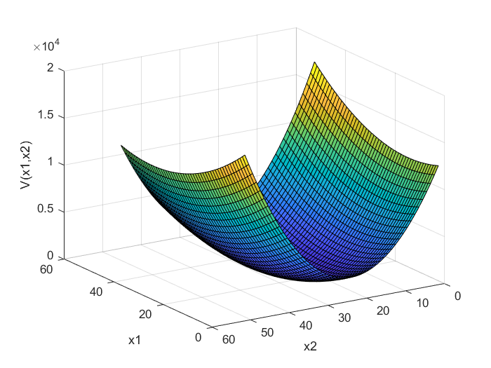 for the
  matrix in (8).
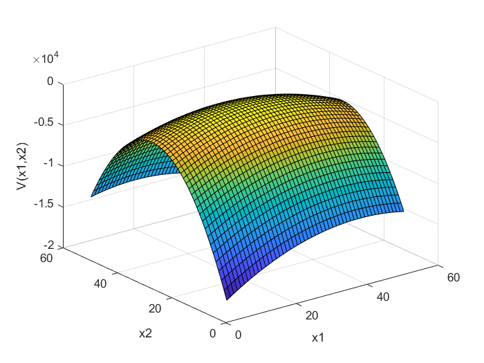 for the
  matrix in (8).
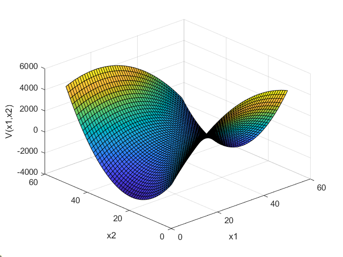 for the
  matrix in (8).
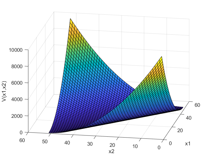 for the
  matrix in (8).
The MATLAB code used to generate these plots is given below.
clear,pack,clc
x1=-50:2:50;
x2=-50:2:50;

[X1,X2]=meshgrid(x1,x2);

syms x1s
syms x2s

% P1 - positive definite completely symmetric with respect to the zero axis
%P=[1 0; 0  1];
% P2 - positive definite not completely symmetric
% P=[1 -2;1  5];
% P3 - negative definite
%P=[-1 -2;1  -5];
%P4 - indefinite
%P=[-1 -2; 1  2];
%P5 - positive semi-definite
P=[1 1; 1 1];

expression= [x1s x2s]*P*[x1s; x2s];

% print this expression in the command window to see the expanded form of
% the Z function

% use the expanded expression to define a new function
expand(expression)

V= X1.^2+X2.^2+(X1.*X2).*2

figure(1)
surf(V)
xlabel('x1')
ylabel('x2')
zlabel('V(x1,x2)')
Here, we need to mention one important fact about quadratic forms. Notice that in the definition of the quadratic form, given by Eq. (2), it is assumed that the matrix is symmetric. However, many matrices are not symmetric. Is it possible to define quadratic forms for such matrices? The answer is yes, since
(9) 
Consequently, any non-symmetric matrix defines a quadratic form with a symmetric matrix. That is, for any non-symmetric matrix, we can find a quadratic form with a symmetric matrix.
From (7), we can see that the function is quadratic. For this function to be positive definite, the matrix has to be a positive definite matrix. The symmetric real matrix is said to be a positive definite matrix if and only if, the following condition is satisfied
(10) 
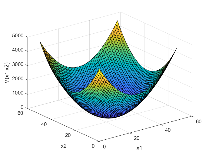
Positive definite quadratic forms corresponding to the positive definite matrices and are illustrated in Figs. 1 and 2. Let us now discuss a test for testing positive definiteness of a matrix. Let us consider the 2D case given by Eq.(7). From this equation, we have:
(11) 
Let us analyze the last expression. Let us assume that  is positive. Then, it is easy to see that the first term is positive for any and different from zero, that is
(12) 
Let us consider the second term
(13) 
The second term is positive for all  if
if
(14) 
The last equation is equivalent to
(15) 
To summarize, the quadratic form (7) is positive definite if
(16) 
On the other hand, consider again the original matrix
(17) 
The number is the leading principal minor of order  (or briefly, the first-order leading principal minor) of the matrix and the expression
  is the leading principal minor of order
  (or briefly, the second-order leading principal minor) of the matrix . The leading principal minors of certain order are determinants of the upper-left submatrices of the matrix. Generally speaking, we can say that the leading principal minor of order
  is the determinant of a matrix obtained by erasing the last
  columns and rows of the matrix
  . Thus, the second-order matrix is positive definite if and only if, its first-order and second-order leading principal minors are positive.
By using this test, we can determine that the matrices and defined in (8) are positive. Consequently, the corresponding quadratic forms that are shown in Fig. 1. and Fig. 2. are positive definite.
Condition for positive definiteness:
Generally speaking, the n-dimensional matrix :
(18) 
is positive definite if and only if
- the first-order leading principal minor is positive, that is, the determinant of the upper left 1-by-1 corner of P is positive:
(19)

- the second-order leading principal minor is positive, that is, the determinant of the upper left 2-by-2 corner of P is positive:
(20)

- the third-order leading principal minor is positive, that is, the determinant of the upper left 3-by-3 corner of P is positive:
(21)

- …
- the determinant of the matrix P is positive (this is the
 -th order leading principal minor)
(22)

This is the Sylvester condition for testing the positive definiteness of a matrix.
Let us apply this test on the following matrix
(23) 
We have
(24) 
Consequently, the matrix is positive-definite.
Let us now state definitions of negative definite, negative semidefinite, positive semidefinite, and indefinite matrices.
Negative definite matrix: A matrix is negative definite if and only if
(25) 
Negative semi-definite matrix: A matrix is negative definite if and only if
(26) 
Positive semi-definite matrix: A matrix is negative definite if and only if
(27) 
Indefinite matrix: A matrix is indefinite if and only if  for some
  , and
, and  for some .
The matrix in (8) is negative definite and the matrix is indefinite. The quadratic form defined for the negative definite matrix is shown in Fig. 3, whereas the quadratic form defined for the indefinite matrix is shown in Fig. 4. The matrix in (8) is positive semi-definite. The quadratic form defined for this matrix is shown in Fig. 5. The quadratic form for the matrix is
(28) 
We see that this quadratic form is positive semi-definite since for  , the quadratic form is zero, and otherwise it is positive (except at
  ). That is, there is some point
  that is different from for which this quadratic form is zero. Next, we state tests for negative definiteness, semi-definiteness, and indefiniteness.
Condition for negative definiteness: A matrix in (18) is negative definite if and only if:
(29) 
That is, the matrix is negative definite if and only if its leading principal minors alternate the sign, starting from the first-order minor that should be negative. Or in other words, the matrix is negative definite if and only if its leading principal minors of odd degree are negative and leading principal minors of even degree are positive.
Condition for indefiniteness: A matrix is indefinite if and only if some leading principal minor is non-zero, but its sign does not follow the pattern for either positive definite or negative definite matrices.
The conditions for positive and negative semidefiniteness are different from the conditions for strict positive and negative definiteness since they involve all principal minors, and not only leading principal minors. Principal minors are simply obtained by erasing certain columns and rows of a matrix and computing the determinant. Here, the process of erasing the columns and rows is not only restricted to the last rows and columns such as in the case of leading principal minors. The column and row numbers should be identical. That is, the indices of deleted rows must be equal to the indices of deleted columns. For example, consider the 3×3 matrix
(30) 
Its second order principal minors are
(31) 
Condition for positive semi-definiteness: A matrix is positive semi-definite if and only if its all principal minors are  .
.
Condition for negative semi-definiteness: A matrix is negative semi-definite if and only if its principal minors of odd degree are  , and principal minors of even degree are .
Asymptotic stability and the Lyapunov equation
Let us assume that the function (2) is positive definite, and this is equivalent to assuming that the matrix is positive definite. In the 2D case, as well as in the n-dimensional case, we can always find the parameters  and
and  to make the matrix positive definite. This means that condition (1) of the Lyapunov stability theorem is satisfied.
Let us now compute the derivative of the function along the trajectories of the system:
(32) 
Next, from (1), we have
(33) 
By substituting (1) and (33) in (32), we obtain
(34) 
Let us define the matrix  :
:
(35) 
Note since the matrix is symmetric, the matrix is also symmetric. By substituting (35) in (34), we obtain
(36) 
Since the matrix is symmetric, we see that if the matrix is positive definite, then the function is negative definite and the equilibrium point is asymptotically stable.
This derivation motivates the introduction of the following theorem.
Theorem about the system stability and the solution of the Lyapunov equation: The real parts of all the eigenvalues of the matrix  of the system (1) are negative (the matrix A is the Hurwitz matrix and the equilibrium point is asymptotically stable), if and only if for any positive definite symmetric matrix there exists a positive definite symmetric matrix that satisfies the Lyapunov equation
(37) 
Furthermore, if the matrix A is Hurwitz, then is the unique solution of (37).
From everything being said, we can deduce a test for testing the stability of the system:
Stability test of the system:
- Select a symmetric positive definite matrix (for example, a diagonal matrix with positive entries).
- Solve the Lyapunov equation (37)
- Test the definiteness of the matrix P. If the matrix is positive definite, the system is asymptotically stable. If the matrix is not positive definite, the system is not asymptotically stable.
Basically, this test enables us to investigate the system stability without computing the eigenvalues of the matrix .