How to Check Observability of a Dynamical System in Python – Fusion of Engineering, Control, Coding, Machine Learning, and Science

In this control engineering and control theory tutorial, we will learn how to numerically check observability of a dynamical system in Python. We will consider both continuous-time and discrete-time systems. In our previous video tutorial, whose link is given here, we introduced the concept of observability. Before reading the tutorial presented below, it is suggested that you go over that tutorial. By reading that tutorial you will obtain a proper understanding of observability of dynamical systems.

The main motivation for creating this video tutorial comes from the fact that in many control engineering books, as well as in lectures available online, you can read that observability of the system is tested by testing the rank of the observability matrix. From a purely theoretical point of view, this is the correct approach for testing observability of linear dynamical systems. The issue with this approach is that in practice, it might happen that the observability matrix has full rank, however, it might be numerically ill-conditioned or very close to a matrix without full rank. That is, it might happen that even if the rank condition for testing observability is satisfied, from the numerical point of view the considered system is unobservable or poorly observable. The correct approach for testing observability is not only to check the matrix rank but also to analyze singular values of the observability matrix. In this tutorial, you will learn how to correctly analyze observability of a linear dynamical system and how to perform numerical observability tests in Python. In this video tutorial, we consider three cases

Observable system
Structurally unobservable system
A system whose observability is parametrized and enables us to demonstrate the transition from the unobservable to the observable system

The YouTube tutorial accompanying this webpage is given below.

Brief Summary of Observability For Continuous-Time Systems

Briefly speaking, the system is observable if and only if we can uniquely reconstruct the system’s (initial) state from the output measurements. We consider a continuous-time linear dynamical system having the following state-space form

(1) $\begin{align*}\dot{\mathbf{x}} & =A\mathbf{x}+B\mathbf{u} \\\mathbf{y} & = C\mathbf{x}\end{align*}$

where

$\mathbf{x}\in \mathbb{R}^{n}$ is the $n$ -dimensional state of the system
$n$ is the state dimension or the order of the system
$\mathbf{y}\in \mathbb{R}^{r}$ is the $r$ -dimensional output of the system. This vector is also known as the observed output.
$\mathbf{u}\in \mathbb{R}^{m}$ is the $m$ -dimensional input of the system. This vector is also known as the control input.
$A\in \mathbb{R}^{n\times n}$ , $B\in \mathbb{R}^{n\times n}$ , and $C\in \mathbb{R}^{r\times n}$ are the system matrices.

Formally speaking, the system is observable if and only if the $n-1$ step observability matrix $O_{n-1}$ has full column rank. That is, if and only if

(2) $\begin{align*}\text{rank}\big(O_{n-1} \big) = n\end{align*}$

where $O_{n-1}$ is the $n-1$ steps observability matrix defined as follows

(3) $\begin{align*}O_{n-1}=\begin{bmatrix} C \\ CA \\ CA^{2} \\ \vdots \\ CA^{n-1} \end{bmatrix}\end{align*}$

Brief Summary of Observability For Discrete-Time Systems

Here, we will summarize the formal observability rank condition for discrete-time systems. This condition is derived in our previous tutorial whose link is given here. We consider a discrete-time linear dynamical system having the following state-space form

(4) $\begin{align*}\mathbf{x}_{k+1} & =A_{d}\mathbf{x}_{k}+B_{d}\mathbf{u}_{k} \\\mathbf{y}_{k} & = C_{d}\mathbf{x}_{k}\end{align*}$

where

$\mathbf{x}_{k}\in \mathbb{R}^{n}$ is the $n$ -dimensional state of the system at the discrete-time instant $k$
$n$ is the state dimension or the order of the system
$\mathbf{y}_{k}\in \mathbb{R}^{r}$ is the $r$ -dimensional output of the system at the discrete-time instant $k$ . This vector is also known as the observed output.
$\mathbf{u}_{k}\in \mathbb{R}^{m}$ is the $m$ -dimensional input of the system at the discrete-time instant $k$ . This vector is also known as the control input.
$A_{d}\in \mathbb{R}^{n\times n}$ , $B_{d}\in \mathbb{R}^{n\times n}$ , and $C_{d}\in \mathbb{R}^{r\times n}$ are discrete-time system matrices.

The observability condition for the discrete-time system has an identical form to the observability condition for the continuous-time systems. Formally speaking, the discrete-time system is observable if and only if the $n-1$ step observability matrix $O_{d,n-1}$ has full column rank. That is, if and only if

(5) $\begin{align*}\text{rank}\big(O_{d,n-1} \big) = n\end{align*}$

where $O_{d,n-1}$ is the $n-1$ steps discrete-time observability matrix defined as follows

(6) $\begin{align*}O_{d,n-1}=\begin{bmatrix} C_{d} \\ C_{d}A_{d} \\ C_{d}A^{2}_{d} \\ \vdots \\ C_{d}A^{n-1}_{d} \end{bmatrix}\end{align*}$

Correct Numerical Test for Testing Observability

From the previous two sections, we have seen that in order to test observability we need to compute the rank of the observability matrix. From a purely theoretical point of view, this is the correct approach for testing observability of linear dynamical systems. The issue with this approach is that in practice, it might happen that the observability matrix has full rank, however, it might be numerically ill-conditioned or very close to a matrix without full rank. That is, it might happen that even if the rank condition for testing observability is satisfied, from the numerical point of view the considered system is unobservable or poorly observable. The correct approach for testing observability is not only to check the matrix rank but also to analyze singular values of the observability matrix.

That is, to truly test observability of a dynamical system, we need to augment the rank test with the analysis of singular values of the observability matrix. The singular values are computed by performing the singular value decomposition:

(7) $\begin{align*}O_{n-1}=U\Sigma V^{T}\end{align*}$

where $U$ and $V$ are orthogonal matrices and $\Sigma$ is the rectangular diagonal matrix (not exactly the square diagonal matrix, instead, it contains a block matrix that is a square diagonal matrix). The matrix $\Sigma$ contains singular values that are ordered from the largest one to the smallest one. That is, by computing the singular value decomposition, we compute the singular values of the observability matrix.

The maximum and minimum singular values of the observability matrix can tell us a lot about the practical observability of the system. If the ratio of the largest and smallest singular values is not large, then we can conclude that the system is numerically observable. On the other hand, if the ratio of the largest and smallest singular values is very large (for example in the order of $10^{12}$ or even larger), then from the practical point of view, the system is not observable. The ratio of the maximum and minimum singular value of a matrix is called the condition number. That is, if the condition number is not large, then the system is numerically observable. On the other hand, if the condition number is large, the system is not numerically observable.

Also, the smallest singular value can be used to test the observability. If the smallest singular value of the observability matrix is close to zero or equal to a very small number, then from the practical point of view the system is not observable. In contrast, if the smallest singular value is not a very small number, then from the practical point of view, the system is observable.

Observability Test in Python – Case I – Observable System

First, we consider an observable system. We consider a mass-spring-damper system shown in the figure below:

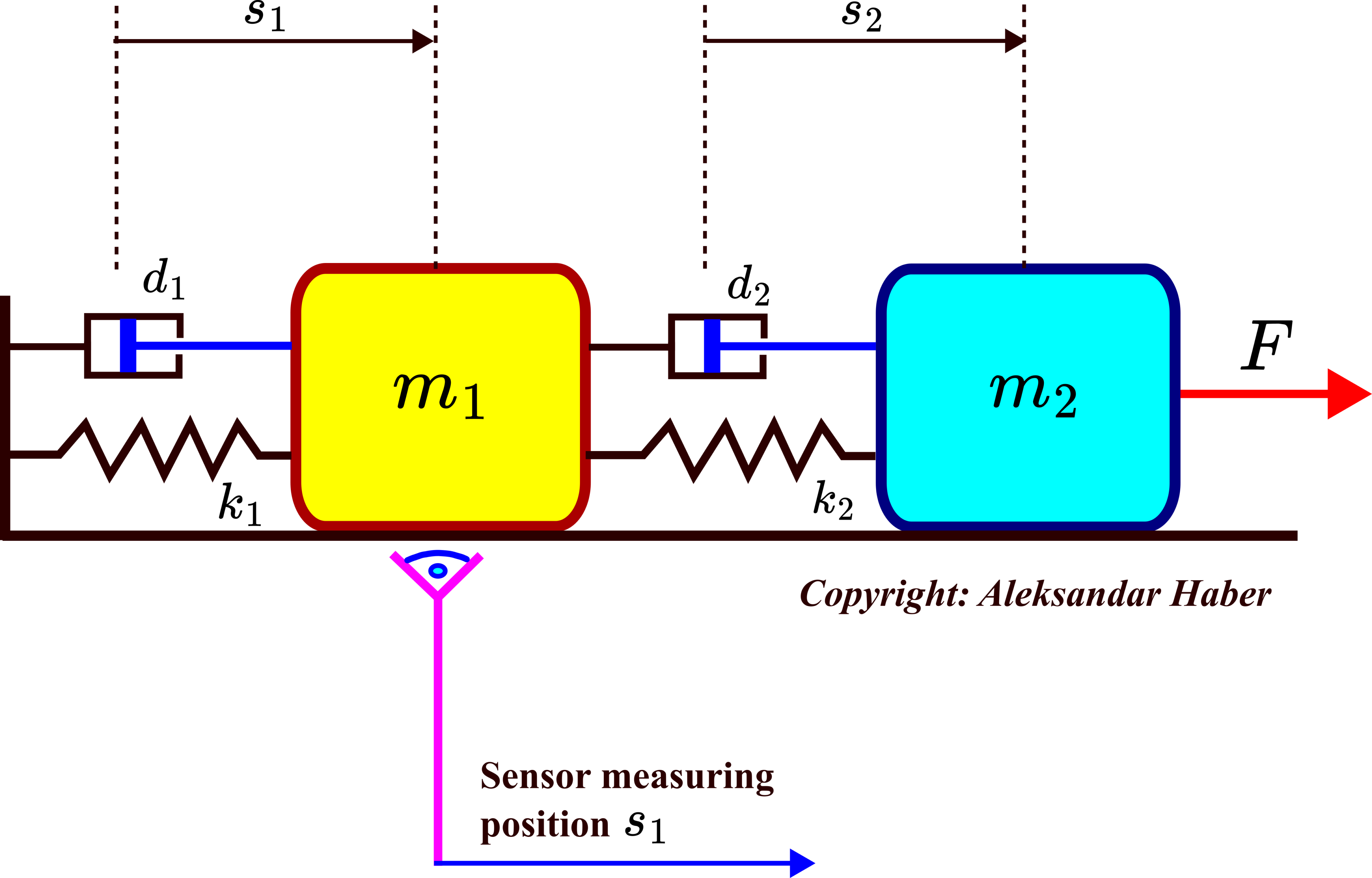
This system consists of two objects that are connected by springs and dampers. This is a prototypical system that can be used to model a large number of dynamical systems, such as mechanical systems exhibiting oscillating behavior, robotic links, car suspension systems, etc. The mass of object 1 is $m_{1}$ . The mass of object two is $m_{2}$ . The parameters $k_{1}$ and $k_{2}$ are spring constants of the first and second springs. The parameters $d_{1}$ and $d_{2}$ are damping constants of the first and second damper. The force $F$ is the external control force applied to the system. The position of the first and second objects are denoted by $s_{1}$ and $s_{2}$ , respectively. The velocities of the first and second objects are denoted by $\dot{s}_{1}$ and $\dot{s}_{2}$ , respectively.

We assume that there is a sensor measuring the position of the first object. That is, we assume that $s_{1}$ is directly observed. We derived a state-space model of this system in our previous tutorial given here. The state-space variables are selected as follows

(8) $\begin{align*}x_{1}=s_{1},\;\; x_{2}=\dot{s}_{1},\;\; x_{3}=s_{2},\;\; x_{4}=\dot{s}_{2}\end{align*}$

The state vector is defined as follows

(9) $\begin{align*}\mathbf{x}=\begin{bmatrix} x_{1} \\ x_{2} \\ x_{3} \\ x_{4} \end{bmatrix}\end{align*}$

The state-space model is given below (for the explanation, see the tutorial whose link is given here):

(10) $\begin{align*}\dot{\mathbf{x}} & =A\mathbf{x}+B\mathbf{u} \\\mathbf{y}& = C\mathbf{x}\end{align*}$

where

(11) $\begin{align*}& \mathbf{x}=\begin{bmatrix}x_{1} \\ x_{2} \\ x_{3} \\ x_{4}\end{bmatrix},\; \mathbf{u}=\begin{bmatrix}F \end{bmatrix},\;\; A=\begin{bmatrix} 0 & 1 & 0 & 0 \\ -\frac{k_{1}+k_{2}}{m_{1}} & -\frac{d_{1}+d_{2}}{m_{1}} & \frac{k_{2}}{m_{1}} & \frac{d_{2}}{m_{1}} \\ 0 & 0 & 0 & 1 \\ \frac{k_{2}}{m_{2}} & \frac{d_{2}}{m_{2}} & -\frac{k_{2}}{m_{2}} & -\frac{d_{2}}{m_{2}} \end{bmatrix},\;\; \\ & B=\begin{bmatrix} 0 \\ 0 \\ 0 \\ \frac{1}{m{2}} \end{bmatrix},\;\; C=\begin{bmatrix}1 & 0 & 0 & 0 \end{bmatrix}\end{align*}$

The following Python code is used to test observability of this system

# -*- coding: utf-8 -*-
"""
Observability test in Python
Author: Aleksandar Haber
Date: November 2023
CASE I: Observable System
"""
import numpy as np
###############################################################################
#       function that creates the observability matrix
###############################################################################

def observabilityMatrix(Ain,Cin):
    (r,n)=Cin.shape
    ObsMatrix=np.zeros(shape=(r*n,n))
    powerA=np.eye(n,n)
    for i in range(n):
        ObsMatrix[r*i:r*(i+1),:]=np.matmul(Cin,powerA)
        powerA=np.matmul(powerA,Ain)
    return ObsMatrix

###############################################################################

###############################################################################    
#                 Case I - Observable System
###############################################################################    
# define the system parameters
m1=2  ; m2=3   ; k1=100  ; k2=200 ; d1=1  ; d2=5; 
 
# define the continuous-time system matrices
A=np.array([[0, 1, 0, 0],
             [-(k1+k2)/m1 ,  -(d1+d2)/m1 , k2/m1 , d2/m1 ], 
             [0 , 0 ,  0 , 1], 
             [k2/m2,  d2/m2, -k2/m2, -d2/m2]])
B=np.array([[0],[0],[0],[1/m2]])
C=np.array([[1, 0, 0, 0]])
D=np.array([[0]])
 
obsM=observabilityMatrix(A,C)

# check the rank 
np.linalg.matrix_rank(obsM)

#compute the singular value decomposition
# of the observability matrix 

U,S,V=np.linalg.svd(obsM)
# compute the singular value decomposition
# first approach 
print(np.linalg.cond(obsM))
#second approach 
print(S.max()/S.min())

The Python script presented above first defines a function for creating the observability matrix. Then, it creates the system matrices. We use the NumPy function “np.linalg.matrix_rank” to test the rank of the observability matrix. As expected, the matrix rank is equal to 4. This means that the system is observable since the order of the system is equal to $4$ . Then, we investigate practical observability of the system by computing the singular value decomposition of the observability matrix. Finally, we compute the condition number of the observability matrix. The computer condition number is $1785.13$ . Since this condition number is not large, that is, it is not in the order of $10^{12}$ or in the order of a larger number, we conclude that the system is practically observable.

Next, to illustrate that the condition number is a good measure of the system’s observability, we add an additional observed output to our system. That is, besides the state variable $x_{1}$ (position of the first object), we also assume that the state variable $x_{3}$ is observed (position of the second object). We expect that after this modification, the system will become more observable since we can observe an additional state variable, and consequently, it will be easier to reconstruct the complete state vector by using two directly observed state variables. The Python script given below performs this modification and tests observability.


# now change the matrix C
Cnew=np.array([[1, 0, 1, 0]])
obsMnew=observabilityMatrix(A,Cnew)

# check the rank 
np.linalg.matrix_rank(obsMnew)

#compute the singular value decomposition
# of the observability matrix 

Unew,Snew,Vnew=np.linalg.svd(obsMnew)
# compute the condition number
# first approach 
print(np.linalg.cond(obsMnew))
#second approach 
print(Snew.max()/Snew.min())

The condition number of the modified observability matrix is $379.713$ . We can observe that the condition number decreased compared to the previous case. As expected, this implies that the modified system is more observable than the first system.

Observability Test in Python – Case II – Unobservable System

Here, we perform tests on an unobservable system. We consider the following system

(12) $\begin{align*}\dot{\mathbf{x}} & =A\mathbf{x} \\\mathbf{y} & =C\mathbf{x}\end{align*}$

where

(13) $\begin{align*}A=\begin{bmatrix} A_{1} & 0 \\ 0 & A_{2} \end{bmatrix} \\C=\begin{bmatrix} 1 & 0 & 0 & 0 \end{bmatrix}\end{align*}$

where $A_{1},A_{2}\in \mathbb{R}^{2\times 2}$ are two $2$ by $2$ random matrices. The system is not observable due to the following two reasons

The complete system can be seen as the coupling of two second-order systems that are decoupled. The dynamics of the first system is described by the matrix $A_{1}$ and the dynamics of the second system is described by $A_{2}$ . The matrix $A$ is a block diagonal matrix which means that two systems are decoupled.
We are only measuring the state of the first system. That is, the matrix $C$ has one only at the first position.

The Python script is given below.

"""
Observability test in Python
Author: Aleksandar Haber
Date: November 2023
CASE 2: Unobservable system

"""
import numpy as np
###############################################################################
#       function that creates the observability matrix
###############################################################################

def observabilityMatrix(Ain,Cin):
    (r,n)=Cin.shape
    ObsMatrix=np.zeros(shape=(r*n,n))
    powerA=np.eye(n,n)
    for i in range(n):
        ObsMatrix[r*i:r*(i+1),:]=np.matmul(Cin,powerA)
        powerA=np.matmul(powerA,Ain)
    return ObsMatrix

###############################################################################


###############################################################################    
#                 Case II - Unobservable System
###############################################################################    
# create two decoupled systems 
A2=np.zeros(shape=(4,4))
A2[0:2,0:2]=np.random.randn(2,2)
A2[2:4,2:4]=np.random.randn(2,2)
C2=np.array([[1, 0, 0, 0]])

obsMnew2=observabilityMatrix(A2,C2)

# check the rank 
np.linalg.matrix_rank(obsMnew2)

#compute the singular value decomposition
# of the observability matrix 

Unew2,Snew2,Vnew2=np.linalg.svd(obsMnew2)
# compute the singular value decomposition
# first approach 
print(np.linalg.cond(obsMnew2))
#second approach 
print(Snew2.max()/Snew2.min())

The A matrix of this system is

array([[-0.58458549,  0.50254489,  0.        ,  0.        ],
       [-0.75027269,  0.11005184,  0.        ,  0.        ],
       [ 0.        ,  0.        ,  0.89584881, -0.48266915],
       [ 0.        ,  0.        , -0.57567866, -0.49096135]])

We can see that the system consists of two decouples second order system. The C matrix of this system is

array([[1, 0, 0, 0]])

This C matrix tells us that only the first state variable of the first system is measured. This means that we do not have any information about the states of the second system.

The rank of the observability matrix is equal to 2 . Consequently, the system is not observable. The condition number is infinity since the smallest singular value is equal to 0. That is, the matrix is rank deficient.

Observability Test in Python – Case III – Transition from Unobservable to Observable System

In this case, we parametrize the system output, and we explain how the introduced parameter influences the system observability. We consider the system from Case II given by equations (12) and (13), with one important difference. The output $C$ matrix looks like this

(14) $\begin{align*}C=\begin{bmatrix} 1 & 0 & \delta & 0 \end{bmatrix}\end{align*}$

where $\delta$ is a parameter that we vary. By varying this parameter from $0$ to a larger number, we will have the transition from unobservable to observable systems. We will show that the condition number decreases as the number $\delta$ increases. This means that the system becomes more observable as the parameter delta is increased.

The Python script is given below.

"""
Observability test in Python
Author: Aleksandar Haber
Date: November 2023
CASE 3: Transition from unobservable to observable system

"""
import numpy as np
###############################################################################
#       function that creates the observability matrix
###############################################################################

def observabilityMatrix(Ain,Cin):
    (r,n)=Cin.shape
    ObsMatrix=np.zeros(shape=(r*n,n))
    powerA=np.eye(n,n)
    for i in range(n):
        ObsMatrix[r*i:r*(i+1),:]=np.matmul(Cin,powerA)
        powerA=np.matmul(powerA,Ain)
    return ObsMatrix

###############################################################################


###############################################################################    
#                 Case III - Transition from Unobservable to Observable
###############################################################################    
# create two decoupled systems 
A2=np.zeros(shape=(4,4))
A2[0:2,0:2]=np.random.randn(2,2)
A2[2:4,2:4]=np.random.randn(2,2)
delta=0.00000001
C2=np.array([[1, 0, delta, 0]])

obsMnew2=observabilityMatrix(A2,C2)

# check the rank 
np.linalg.matrix_rank(obsMnew2)

#compute the singular value decomposition
# of the observability matrix 

Unew2,Snew2,Vnew2=np.linalg.svd(obsMnew2)
# compute the singular value decomposition
# first approach 
print(np.linalg.cond(obsMnew2))
#second approach 
print(Snew2.max()/Snew2.min())

For delta=0, the system is not observable and the rank of the observability matrix is $2$ . The condition number is infinity. For delta=0.0000000001, the rank of the observability matrix is 4. However, the condition number is a very large number equal to 54188379445. Despite the fact that the rank of the observability matrix is 4, since the condition number is large, this means that the system is not practically observable. For delta=0.00001, the rank of the observability matrix is 4. The condition number is 1143673. Since this number is not extremely large, we can conclude that the system is numerically observable.

Brief Summary of Observability For Continuous-Time Systems

Brief Summary of Observability For Discrete-Time Systems

Correct Numerical Test for Testing Observability

Observability Test in Python – Case I – Observable System

Observability Test in Python – Case II – Unobservable System

Observability Test in Python – Case III – Transition from Unobservable to Observable System

admin

You might also like

Clear and Graphical Explanation of Signal Convolution with MATLAB Implementation – Digital Signal Processing Tutorial

Quadratic Forms, Positive Definite, Negative Definite, and Semi-Definite Matrices

How To Approximate Expectations and Integrals of Functions by Using the Monte Carlo Method