Control Systems Lecture: Basic Principles of Feedback Control – Fusion of Engineering, Control, Coding, Machine Learning, and Science

In this post, we explain basic principles of feedback control method. The video accompanying this post is given below.

In our previous post (see this post and this post), we have introduced a model of a mass-spring-damper system. This system will be used to motivate and to explain basic principles of feedback control. We are using this system model since it can be used to mathematically model a number of mechanical, electrical, chemical, technological, and physical systems. The sketch of the system is given in the figure below.

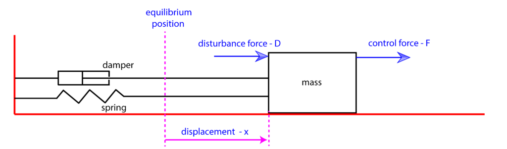
Figure 1: Mass-spring-damper system used to illustrate the basic principles of feedback control.

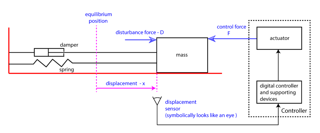
The goal of the control algorithm is to move (steer) the object of the mass $m$ to the desired position, which is denoted by $r$ (reference position). We assume that there is a sensor measuring the object displacement. On the basis of the sensor measurement, and on the basis of the reference (desired) object position, we can compute the control error

(1) $\begin{align*}e(t)=r(t)-x(t)\end{align*}$

where $x(t)$ is the displacement. The controller takes the control error as an input, and on the basis of this control error, it generates the control force $F$ . Since the main purpose of this lecture is to introduce basic principles of feedback control, and in order not to blur the main ideas with additional mathematical perplexities, in this post, we assume a simple form of the control algorithm that is mathematically represented by the following equation

(2) $\begin{align*}F(t)=Ke(t)\end{align*}$

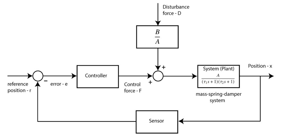
where $K\in \mathbb{R}$ is a control parameter that we need to determine. Since the control force is directly proportional to the control error, this type of controller is referred to as the proportional feedback controller. This feedback control approach as well as other feedback control schemes can be illustrated by a diagram shown in the figure below.

Figure 2: Graphical explanation of the feedback control approach.

The system transfer function model that is explained in the previous post, has the following form.

(3) $\begin{align*} X(s)=W_{1}(s)F(s)+W_{2}(s)D(s)\end{align*}$

where $W_{1}(s)$ and $W_{2}(s)$ are transfer functions defined as follows

(4) $\begin{align*}W_{1}(s)=\frac{A}{(\tau_{1}s+1)(\tau_{2}s+1)}, \; W_{2}(s)=\frac{B}{(\tau_{1}s+1)(\tau_{2}s+1)}\end{align*}$

and where $F(s)$ and $D(s)$ are the Laplace transforms of the control force $F$ and disturbance force $D$ , $X(s)$ is the Laplace transform of the displacement $x(t)$ , and $A,B,\tau_{1}$ and $\tau_{2}$ are system parameters.

The feedback control approach can be graphically represented by the following block diagram.

Figure 3: Block diagram of the feedback control approach.

Let us now investigate the effect of this controller structure on the overall system performance. First, we assume that the reference signal and the disturbance force are constants, and that they are denoted by

(5) $\begin{align*}r(t)=r_{d},\;\; D(t)=D\end{align*}$

That is, we assume that the control objective is to displace the object to the position $r_{d}$ and to keep the object at that position. Next, we take Laplace transforms of the equations (2), (5), and (14):

(6) $\begin{align*}& E(s)=R(s)-X(s) \\& F(s)=KE(s) \\& R(s)=\frac{r_{d}}{s} \\& D(s)=\frac{D}{s}\end{align*}$

By substituting (6) in (3), we obtain

(7) $\begin{align*}& X(s)= W_{1}(s)K\Big(R(s)-X(s)\Big)+W_{2}(s)D(s) \notag \\& \Big(1 + W_{1}(s)K \Big)X(s) =W_{1}(s)KR(s)+W_{2}(s)D(s) \notag \\& X(s)= \frac{W_{1}(s)K}{1 + W_{1}(s)K }R(s)+\frac{W_{2}(s)}{1 + W_{1}(s)K }D(s)\end{align*}$

and the final expression

(8) $\begin{align*}X(s)= \frac{W_{1}(s)K}{1 + W_{1}(s)K }\cdot \frac{r_{d}}{s}+\frac{W_{2}(s)}{1 + W_{1}(s)K}\cdot \frac{D}{s}\end{align*}$

Let us assume that the controller $K$ is selected such that the poles of the transfer function

(9) $\begin{align*} \frac{W_{1}(s)K}{1 + W_{1}(s)K },\;\;\; \frac{W_{2}(s)}{1 + W_{1}(s)K }\end{align*}$

are in the left-half od the s-plane. That is, we assume that the equilibrium point of the system is asymptotically stable. Under this assumption, we can apply the final value theorem. The final value theorem states that if the poles of the expression $sX(s)$ are in the left part of the s-plane, then we have

(10) $\begin{align*} x_{ss}=\lim_{t\rightarrow \infty} x(t) =\lim_{s \rightarrow 0} sX(s) \end{align*}$

where $x_{ss}$ is the steady-state object position. By applying this theorem to (8) we obtain

(11) $\begin{align*}& x_{ss}=\lim_{t\rightarrow \infty} x(t) = \lim_{s \rightarrow 0} sX(s) \notag \\& x_{ss} = \lim_{s \rightarrow 0} \frac{W_{1}(s)K}{1 + W_{1}(s)K } r_{d}+\lim_{s \rightarrow 0} \frac{W_{2}(s)}{1 + W_{1}(s)K}D \\& x_{ss} = \frac{ \lim_{s \rightarrow 0} W_{1}(s)K}{\lim_{s \rightarrow 0}\Big(1 + W_{1}(s)K\Big) } r_{d}+\frac{\lim_{s \rightarrow 0} W_{2}(s)}{\lim_{s \rightarrow 0}\Big(1 + W_{1}(s)K\Big)}D \\ \end{align*}$

Let us now evaluate these limit values. From (4), we obtain

(12) $\begin{align*} & \lim_{s \rightarrow 0} W_{1}(s)K = \lim_{s \rightarrow 0} \frac{AK}{(\tau_{1}s+1)(\tau_{2}s+1)}= AK \notag \\ & \lim_{s \rightarrow 0}\Big(1 + W_{1}(s)K\Big) = 1+\lim_{s \rightarrow 0}W_{1}(s)K=1+AK \notag \\& \lim_{s \rightarrow 0} W_{2}(s) = \lim_{s \rightarrow 0} \frac{B}{(\tau_{1}s+1)(\tau_{2}s+1)} = B \end{align*}$

Substituting these expressions in the last equation of (11), we obtain

(13) $\begin{align*}x_{ss} = \frac{AK}{1+AK}\cdot r_{d} + \frac{B}{1+AK} \cdot D\end{align*}$

Let us now compute the steady-state error:

(14) $\begin{align*}& e_{ss}= r_{d}-x_{ss}=r_{d}-\frac{AK}{1+AK}\cdot r_{d} - \frac{B}{1+AK} \cdot D \end{align*}$

(15) $\begin{align*}e_{ss} = r_{d}-x_{ss}=\Big(\frac{1}{1+AK} \Big) r_{d} - \frac{B}{1+AK} \cdot D\end{align*}$

On the other hand, from our previous post, it follows that the open-loop steady-state position and error are given by:

(16) $\begin{align*} x_{ss}^{OL} = AK \cdot r_{d}+ B \cdot{D} \end{align*}$

(17) $\begin{align*} e_{ss}^{OL} = (1-AK) \cdot r_{d} - B \cdot{D} \end{align*}$

This analysis enables us to draw the following conclusions.

Benefits of high feedback gain. From (13) and (15) we can observe that if $AK>>1$ and $AK>B$ , then
(18) $\begin{align*}\frac{AK}{1+AK} \approx 1, \;\; \frac{B}{1+AK}\approx 0, \;\; \frac{1}{1+AK}\approx 0 \end{align*}$

This implies that
(19) $\begin{align*}x_{ss}\approx r_{d}, \;\; e_{ss}\approx 0\end{align*}$

That is if the value of the product $AK$ is high, then, we achieve:

a) Small steady-state error. This means that our object will practically reach the desired destination.

b) Good disturbance rejection.

The number $AK$ is the gain of the feedback loop. This can be seen in Figure 3. Consequently, this control approach is called the high-feedback gain control approach. As we will see in our next post, another benefit of increasing the feedback gain is that we can in some sense increase the system robustness. However, for certain classes of systems, high-gain feedback can destabilize the control system! This will be explained in one of our future posts (links will be provided later). In practice, we often need to perform loop shaping to achieve optimal values of controller parameters.
If we compare the open-loop and closed-loop steady-state displacements and errors, we conclude that with feedback control we are able to attenuate the effect of disturbances on our system. Furthermore, we will see in our future posts that feedback control is more robust than the open-loop control.

There are also other benefits and trade-offs in feedback control. These properties of feedback control will be explained in our next posts.

admin

You might also like

Model Predictive Control (MPC) Tutorial 2: Unconstrained Solution for Linear Systems and Implementation in C++ from Scratch by Using Eigen C++ Library

Clear Explanation of the Value Function and Its Bellman Equation – Reinforcement Learning Tutorial

Python Control Systems Library Tutorial 1: Define Transfer Functions and Compute Step, Initial State, and Input Responses