Control Systems Lecture: From Differential Equations to Transfer Functions and Response Simulation in MATLAB – Fusion of Engineering, Control, Coding, Machine Learning, and Science

We can describe a linear system dynamics using differential equations or using transfer functions. In this post, we will learn how to

1.) Transform an ordinary differential equation to a transfer function.
2.) Simulate the system response to different control inputs using MATLAB.

The video accompanying this post is given below.

We have explained that the dynamics of a large number of second-order systems can be generically represented as mass-spring-damper systems. Consequently, in this post we consider a generic mass-spring-damper system

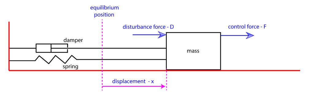
Figure 1: Mass-spring system with control and disturbance force

In our previous post, we have explained how to derive a differential equation describing the system dynamics. The system dynamics has the following form:

(1) $\begin{align*}m\ddot{x}+k_{d}\dot{x}+k_{s}x=bF+cD\end{align*}$

where $x$ is the displacement from the equilibrium point, $m$ is mass, $k_{d}$ is a damping coefficient, $k_{s}$ is a spring constant, $b$ is a control input constant, $c$ is a disturbance constant, $F$ is a control force, and $D$ is a disturbance constant. For simplicity, we will write (1) as follows

(2) $\begin{align*}\ddot{x}+\frac{k_{d}}{m}\dot{x}+\frac{k_{s}}{m}x=\frac{b}{m}F+\frac{c}{m}D\end{align*}$

Let us introduce the following notation. If $x(t)$ is a time-domain variable then its Laplace transform is denoted by $X(s)$ , where $s$ is a complex variable. Similarly, Laplace transforms of $F(t)$ and $D(t)$ are denoted by $F(s)$ and $D(s)$ . Let us recall an important Laplace transform relation. If $x^{(n)}(t)$ is the $n$ -th derivative of $x(t)$ , then

(3) $\begin{align*}&\mathcal{L}\{x^{(n)}(t)\}=s^{n}X(s)-s^{n-1}x(0)-s^{n-2}x^{(1)}(0)-s^{n-3}x^{(2)}(0)- \notag \\ &\ldots -x^{(n-1)}(0)\end{align*}$

where $x(0), x^{(1)}(0),\ldots,x^{(n-1)}(0)$ is the initial condition and first, second, …, and $n$ -th derivative of $x(t)$ evaluated at $t=0$ . Applying this rule to (2), we obtain

(4) $\begin{align*}s^{2}X(s)-sx(0)-x^{(1)}(0)+\frac{k_{d}}{m}sX(s)-x(0)+\frac{k_{s}}{m}X(s) = \notag \\\frac{b}{m}F(s)+\frac{c}{m}D(s)\end{align*}$

In order to define a transfer function, we need to set the initial condition and all of its derivatives to zero. Under this assumption from (4), we have

(5) $\begin{align*}\Big(s^{2}+\frac{k_{d}}{m}s+\frac{k_{s}}{m} \Big)X(s)=\frac{b}{m}F(s)+\frac{c}{m}D(s)\end{align*}$

(6) $\begin{align*}X(s)=W_{1}F(s)+W_{2}D(s)\end{align*}$

where $W_{1}(s)$ is a transfer function from the control force to the displacement

(7) $\begin{align*}W_{1}(s)=\frac{\frac{b}{m}}{s^{2}+\frac{k_{d}}{m}s+\frac{k_{s}}{m}}\end{align*}$

and $W_{2}(s)$ is the transfer function from the disturbance force to the displacement

(8) $\begin{align*}W_{2}(s)=\frac{\frac{c}{m}}{s^{2}+\frac{k_{d}}{m}s+\frac{k_{s}}{m}}\end{align*}$

In control systems, we often use two ways for representing transfer functions. Both ways are based on the factorization of polynomials in denominators. Let us recall the completition of squares from calculus. How to factorize the following polynomial?

(9) $\begin{align*}P(s)=s^{2}+bs+c\end{align*}$

Well, we can use the completition of squares trick. We can write

(10) $\begin{align*}P(s)=s^{2}+2\frac{1}{2}bs+\frac{1}{4}b^{2}-\frac{1}{4}b^{2}+c \notag \\P(s)=(s+\frac{b}{2})^{2}-(\frac{1}{4}b^{2}-c) \\\end{align*}$

Next, using the following fact $p^{2}-q^{2}=(p-q)(p+q)$ , we can write

(11) $\begin{align*}P(s)=\Big(s+\frac{b}{2} - \sqrt{\frac{b^{2}-4c}{4}}\Big)\Big(s+\frac{b}{2} + \sqrt{\frac{b^{2}-4c}{4}}\Big) \\P(s)=\Big(s-\big( \frac{-b+\sqrt{b^{2}-4c}}{2} \big) \Big)\Big(s-\big( \frac{-b-\sqrt{b^{2}-4c}}{2} \big)\Big)\end{align*}$

On the other hand, the solutions of the quadratic equation $P(s)=0$ are

(12) $\begin{align*}s_{1,2}=\frac{-b\pm \sqrt{b^{2}-4c}}{2}\end{align*}$

From the last two equations, we conclude that we can factorize the polynomial (9), by computing its zeros $s_{1}$ and $s_{2}$ , and then writting

(13) $\begin{align*}P(s)=(s-s_{1})(s-s_{2})\end{align*}$

Let us now use these insigths to factorize the transfer function (7) and (8). First, we compute zeros of the denominator

(14) $\begin{align*}\tilde{s}_{1,2}=\frac{-\frac{k_{d}}{m}\pm \sqrt{\frac{k_{d}^{2}}{m^{2}}-4\frac{k_{s}}{m}}}{2}\end{align*}$

and consequently, we can write

(15) $\begin{align*}W_{1}=\frac{\frac{b}{m}}{(s-\tilde{s}_{1})(s-\tilde{s}_{2})}\end{align*}$

and

(16) $\begin{align*}W_{2}=\frac{\frac{c}{m}}{(s-\tilde{s}_{1})(s-\tilde{s}_{2})}\end{align*}$

These transfer function representations are important since they directly reveal the system poles. Next, we explain another way for expressing the transfer function. Namely, we can write

(17) $\begin{align*}W_{1}=\frac{\frac{b}{m}}{(-\tilde{s}_{1})(-\tilde{s}_{2})(\frac{1}{-\tilde{s}_{1}}s+1)(\frac{1}{-\tilde{s}_{2}}s+1)}\end{align*}$

By substituting (14) in (17), we obtain

(18) $\begin{align*}W_{1}=\frac{A}{(\tau_{1}s+1)(\tau_{2}s+1)}\end{align*}$

where $A=\frac{b}{k_{s}}$ and $\tau_{1}=\frac{-1}{\tilde{s}_{1}}$ and $\tau_{2}=\frac{-1}{\tilde{s}_{2}}$ . Similarly, we obtain

(19) $\begin{align*}W_{2}=\frac{B}{(\tau_{1}s+1)(\tau_{2}s+1)}\end{align*}$

where $B=\frac{c}{k_{s}}$ .

These forms of transfer function representations are important since they enable us to easily read the system steady-state gains $A$ and $B$ .

There are at least two ways for defining transfer functions in MATLAB. Here is the first way.

% define system parameters
% mass 
m=10
% damping 
kd=1
% spring constant
ks=100

% control force constant
b=1

% disturbance constant
c=0.1

% Defining transfer functions

% control to position transfer function
% numerator 
num1=[b/m];
% denominator
den1=[1 kd/m ks/m]
W1=tf(num1,den1)

% disturbance to position transfer function
% numerator
num2=[c/m];
den2=[1 kd/m ks/m]
W2=tf(num2,den2)

% compute poles of transfer functions 

pole(W1)

% check the computations, these should be poles
s1=(-(kd/m)+sqrt( (kd/m)^2 -4*(ks/m) ))/2
s2=(-(kd/m)-sqrt( (kd/m)^2 -4*(ks/m) ))/2

Here is the second method relying on the MATLAB symbolic toolbox.

% another way for defining transfer functions

tau1= 1/(-s1);
tau2= 1/(-s2);

A=b/ks;
B=c/ks;

s = tf('s');

W1_other_form=A/((tau1*s+1)*(tau2*s+1))
W2_other_form=B/((tau1*s+1)*(tau2*s+1))

pole(W2_other_form)
pole(W2)

Next, we compute step responses of the two transfer functions. The code is given below.

% compute the system step response

% define the simulation time

simulation_time=0:0.1:100;

y1=step(W1,simulation_time)
figure(1)
plot(simulation_time,y1)
y2=step(W2,simulation_time)
figure(2)
plot(simulation_time,y2)

The two computed step responses are given in figures below.

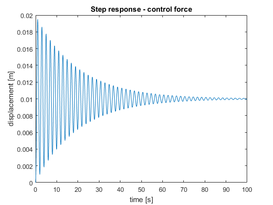
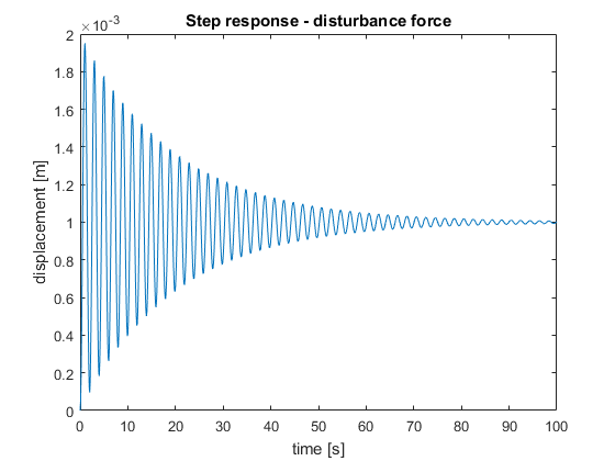
Figure 2: Step response from the control force to the displacement.

Figure 3: Step response from the control disturbance force to displacement.

We can observe that both simulated step responses approximately end at the values that correspond to the steady-state gains of the system. Namely, in the case of $W_{1}$ , we have

(20) $\begin{align*} x_{ss}=\lim_{s\rightarrow 0} s \frac{A}{(\tau_{1}s+1)(\tau_{2}s+1)} \frac{1}{s}= A \end{align*}$

where $A=\frac{b}{k_{s}}$ . In our case $A=0.01$ and this value matches the results shown in Figure 2. The similar conclusion can be derived for the case of $W_{2}$ .

admin

You might also like

Feedback Linearization and Control of the Fluid Level in a Tank (Reservoir) – Simulink and MATLAB Implementation.

Interpolation of Function Values in MATLAB

2. Introduction to Pandas structures: Series and DataFrame structures