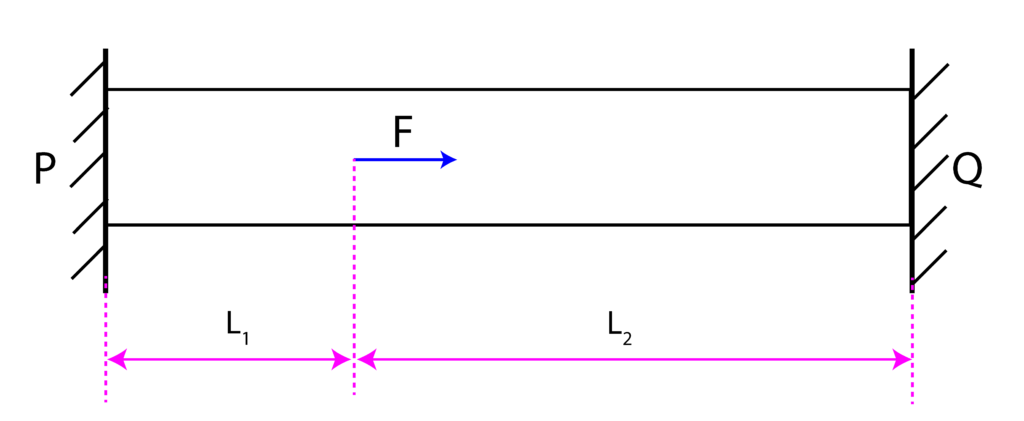
Statically Indeterminate Problem (Axial Deformation) – Fusion of Engineering, Control, Coding, Machine Learning, and Science

Example 1:
Consider the axial member constrained between two planes $P$ and $Q$ . The cross-section area is $A$ and the modulus of elasticity $E$ are given. A numerical value of the force $F$ acting at the distance $L_{1}$ from the plate $P$ is also given. Assuming that $L_{1}$ and $L_{2}$ are known, determine the reaction forces $R_{P}$ and $R_{q}$ .

Example 1: Statically indeterminate problem.

Solution:

The first step is to construct the free body diagram. The free-body diagram is given in the figure below. Notice here that we have assumed the directions of the forces $R_{P}$ and $R_{Q}$ . If we obtain negative values of these forces, then the actual direction of these forces is opposite from the assumed directions.

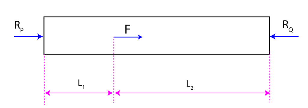
Assuming that the positive direction is the direction of the force $F$ , the static equilibrium condition is

(1) $\begin{align*}R_{P}+F-R_{Q}=0\end{align*}$

This is a single equation with two unknowns $R_{P}$ and $R_{Q}$ . Consequently, we cannot uniquely solve this equation. To solve this equation, we need an additional equation. This equation is a deformation equation. Namely, since the member is constrained between two parallel plates, it cannot deform, and consequently:

(2) $\begin{align*}\Delta L_{\text{total}} = 0\end{align*}$

To compute the total deformation and to set it to zero, we need internal force diagrams. Figure 2 below shows the internal force diagrams. We will briefly revise the procedure for computing internal force diagrams. For additional explanations on how to construct an internal force diagram, see this lecture.

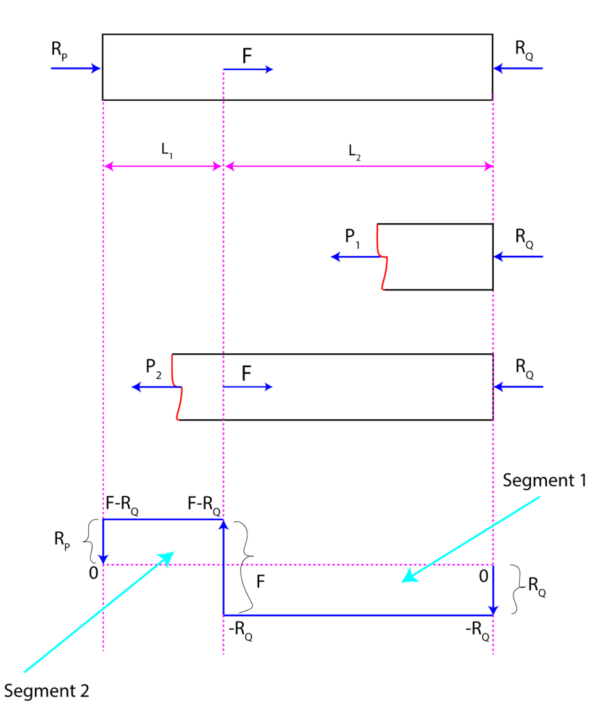
Figure 3: Construction of the internal force diagram.

Let us compute the internal force for Segment 1. Assuming that the positive direction is in the direction of the internal force $P_{1}$ , the static equilibrium condition is

(3) $\begin{align*}P_{1}+R_{Q}=0,\;\; P_{1}=-R_{Q}\end{align*}$

On the other hand, the static equilibrium condition for Segment 2 is

(4) $\begin{align*}P_{2}-F+R_{Q}=0,\;\; P_{2}=F-R_{Q}\end{align*}$

The internal force diagram is shown in the last subfigure of Fig. 3. Once we have determined the internal force diagram, we can compute the total deformation using the principle explained in the previous lecture given here.

We have

(5) $\begin{align*}\Delta L_{\text{total}}= \Delta \text{Segment}_{1}+ \Delta \text{Segment}_{2} =0\end{align*}$

where

(6) $\begin{align*}\Delta \text{Segment}_{1} =\frac{( -R_{Q} ) L_{2}}{EA},\;\; \Delta \text{Segment}_{2} =\frac{( F-R_{Q} ) L_{1}}{EA} \end{align*}$

By substituting these two equations in Eq.(5), we obtain

(7) $\begin{align*} \Delta L_{\text{total}} = \frac{( -R_{Q} ) L_{2}}{EA} + \frac{( F-R_{Q} ) L_{1}}{EA} =0 \notag \\ -R_{Q} L_{2} + ( F-R_{Q} ) L_{1} =0 \end{align*}$

where the second equation is obtained by multiplying the first equation with $EA$ . From the second equation, we obtain

(8) $\begin{align*}F L_{1} =R_{Q} (L_{1}+L_{2})\notag \\ R_{Q} = F \frac{L_{1}}{ L_{1}+L_{2} }\end{align*}$

Next, we substitute the computed $R_{Q}$ in Eq.(1). As the result, we obtain

(9) $\begin{align*} & R_{P}=R_{Q}-F \notag \\& R_{P}= F \frac{L_{1}}{ L_{1}+L_{2} } - F = \frac{F L_{1} - F( L_{1}+L_{2} ) }{ L_{1}+L_{2} } \notag \\ & R_{P}= - F \frac{L_{2}}{L_{1}+L_{2}}\end{align*}$

The fact that we have obtained the negative value of $R_{P}$ , means that the direction of $R_{p}$ is different from the direction assumed while constructing the free-body diagram in Fig. 2 . The problem is solved.

admin

You might also like

Phase Portraits of State-Space Models and Differential Equations in Python

Time Propagation of State Vector Expectation and State Covariance Matrix of Linear Dynamical Systems – Intro to Kalman Filtering

Undamped Linear Harmonic Oscillator