Deformation of Members Under Axial Loading – Fusion of Engineering, Control, Coding, Machine Learning, and Science

In this lecture, we explain how to calculate the deformation of objects under the action of axial force. A YouTube video accompanying this lecture is given below.

Consider figure 1 presented below.

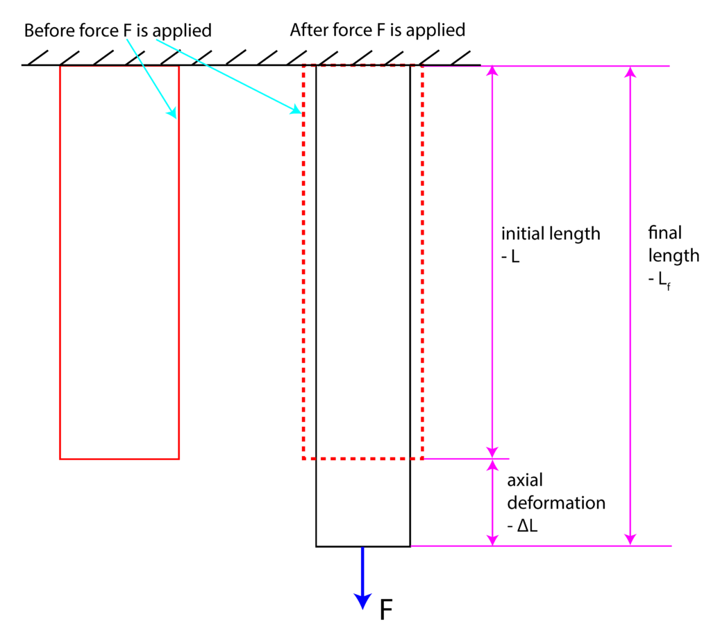
Deformation under the action of axial force $F$ .

Let the cross-section area of the element be denoted by $A$ . Then, the normal stress $\sigma$ is defined by

(1) $\begin{align*}\sigma=\frac{F}{A}\end{align*}$

where $F$ is the applied axial force. Here it should be kept in mind that the stress is defined as

(2) $\begin{align*}\sigma = \frac{\text{internal force}}{\text{cross section area}} = \frac{P}{A}\end{align*}$

where $P$ is the internal force. Consequently, since $P=F$ , we obtain (1). On the other hand, if the stress inside of the material does not exceed the proportional limit that is in the elastic deformation range, then Hooke’s law applies, and we have

(3) $\begin{align*}\sigma = E \varepsilon\end{align*}$

where $E$ is the modulus of elasticity and $\varepsilon$ is the strain, defined by

(4) $\begin{align*}\varepsilon = \frac{\Delta L}{L}\end{align*}$

By substituting (1) and (4) in (3), we obtain

(5) $\begin{align*}\Delta L = \frac{F \cdot L}{E \cdot A}\end{align*}$

That is, the deformation $\Delta L$ is proportional to the applied force and the initial length, and inversely proportional to the modulus elasticity $E$ and cross-section area $A$ . Here it should be emphasized that the developed formula is only valid for the situation illustrated in Fig. 1. In a more complex scenario, we can apply a modified formula. Basically, let us assume that an object consists of segments (that weill be defined later). Then, deformation of a segment is defined by

(6) $\begin{align*}&\text{segment deformation} \notag \\& = \frac{(\text{internal force in a segment})\cdot (\text{initial length of a segment})}{(\text{modulus of elasticity of a segment})\cdot (\text{cross-section area of a segment})}\end{align*}$

Then, total deformation is a sum of deformations of segments.

A segment is defined as a piece of an object for which the cross-section area, internal force, and modulus of elasticity are constant.

Let us illustrate this principle with the following example.

Example 1: Consider the object that is deformed by the system of forces. If the values of $F$ , $E$ , $L$ , and $A$ are given, compute the total deformation of the object.

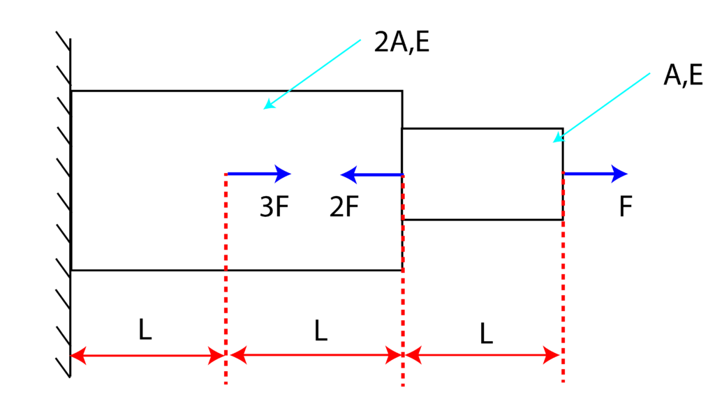
Example 1: object deformed by the system of axial forces.

The first step when solving problems of this type is to construct the internal force diagram. So, let us start from the right side (when sitting in your chair and looking at the screen).

We perform an imaginary cut shown in Figure 2.

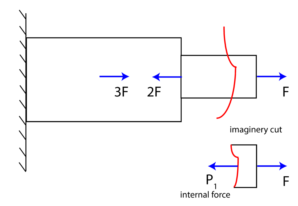
By assuming that the positive direction is in the direction of the internal force $P_{1}$ , the static equilibrium equation is

(7) $\begin{align*}P_{1}-F=0,\;\;\; P_{1}=F\end{align*}$

Then, the second imaginary cut is placed after the action of the force $2F$ . That is, as we move from the right to the left side of the object, the internal force will change since there is external force $2F$ acting on the body. This imaginary cut is shown in Fig. 3 below.

Again, by assuming that the positive direction is in the direction of the internal force $P_{2}$ , the static equilibrium condition takes the following form

(8) $\begin{align*}P_{2}+2F-F=0,\;\; P_{2}=-2F+F,\;\; P_{2}=-F\end{align*}$

That is, we obtained that $P_{2}=-F$ . This means that the internal force has an opposite sign with respect to the sign assumed in Fig. 3.

Finally, as we move again from right to left, we reach the action point of the force $3F$ , and consequently, the internal force changes. This situation is illustrated in Fig. 4 below.

Assuming that the positive direction is in the direction of the internal force $P_{3}$ , the static equilibrium equation produces

(9) $\begin{align*}P_{3}-3F+2F-F=0,\;\; P_{3}=2F \end{align*}$

Now taking into account Eqs. (7), (8), and (9), we can construct an internal force diagram that is shown in Fig. 5 below.

The internal force diagram reveals a lot of information about our object. We can see that the jumps correspond to the external forces. For example, between the segment I and II, we see a jump of $2F$ (absolute value) and that jump is actually equal to the external force. The internal force diagram must start from zero and it must end at zero. We can observe a jump of $2F$ toward zero at the end of segment III. This jump actually corresponds to the reaction force at the point $C$ . Namely, assuming the reaction force direction shown in Fig. 5, and assuming that the positive direction is in the direction of the external force $F$ acting at the beginning of segment I, the static equilibrium equation has the following form

(10) $\begin{align*}F-2F+3F-R_{C}=0,\;\; R_{C}=2F \end{align*}$

Now, the total deformation is equal to

(11) $\begin{align*}\Delta L_{\text{total}}= \Delta L_{I} + \Delta L_{II} + \Delta L_{III} \end{align*}$

where $\Delta L_{I}$ , $\Delta L_{II}$ , and $\Delta L_{III}$ are deformations of the segments $I$ , $II$ , and $III$ . To obtain the deformation for every segment, we just read an internal force from the internal force diagram shown in Fig. 5, and we substitute this value in Eq. (6), as well as values for the cross-section area, length, and modulus of elasticity of the segment. Thus we obtain

(12) $\begin{align*}\Delta {L}_{I} =\frac{F L}{E A} \\ \Delta {L}_{II} =\frac{-F L}{E 2A} \\ \Delta {L}_{III} =\frac{2F L}{E 2A} \end{align*}$

So, the total deformation is

(13) $\begin{align*}& \Delta L_{\text{total}} = \frac{F L}{E A} - \frac{F L}{2E A} + 2\frac{F L}{2E A} \\ & \Delta L_{\text{total}} = \frac{F L}{E A} - \frac{F L}{2E A} + \frac{F L}{E A} \\& \Delta L_{\text{total}} =\frac{3}{2} \frac{F L}{E A} \end{align*}$

admin

You might also like

Easy Explanation of Batch Gradient Descent Method with Python Implementation

Clear Explanation of the Value Function and Its Bellman Equation – Reinforcement Learning Tutorial

Linear Quadratic Regulator (LQR) for Non-Zero Set-Points in Python by Using Control Systems Library