Easy-to-Understand Explanation of the Stochastic Gradient Descent Algorithm with Python Implementation from Scratch – Fusion of Engineering, Control, Coding, Machine Learning, and Science

In this tutorial, we provide an easy-to-understand explanation of the stochastic gradient descent algorithm. In addition, we explain how to implement this algorithm from scratch in Python. A YouTube tutorial accompanying this tutorial is given below.

Before we explain the stochastic gradient method, it is very important to understand the concept of gradient and the concept of batch gradient descent.

What is a Gradient?

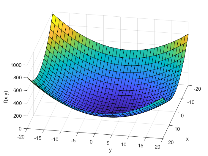
Let us first explain the mathematical concept of a gradient. Let us consider the following function

(1) $\begin{align*}f(x,y)=(x-2)^{2}+(y-2)^{2}\end{align*}$

where $x$ and $y$ are independent variables, and $f(x,y)$ is a real scalar value. This function is illustrated in the figure below.

Now, the question is:

What is the gradient of this function at a certain point?

From the mathematical point of view, the gradient is a vector defined by the following equation

(2) $\begin{align*}g(x,y)=\nabla f(x,y)=\begin{bmatrix} \frac{\partial f}{\partial x} \\ \frac{\partial f}{\partial y} \end{bmatrix} \end{align*}$

where

$\nabla$ (nabla) is a symbol transforming f into the gradient
$g(x,y)$ is the gradient vector
$\frac{\partial f}{\partial x}$ and $\frac{\partial f}{\partial y}$ are the partial derivatives of $f$ with respect to $x$ and $y$ .

Let us compute the gradient of the function (1). The gradient is given by the following equation

(3) $\begin{align*}g(x,y)=\nabla f(x,y)=\begin{bmatrix} \frac{\partial f}{\partial x} \\ \frac{\partial f}{\partial y} \end{bmatrix} =\begin{bmatrix} 2(x-2) \\ 2(y-2) \end{bmatrix}\end{align*}$

The gradient at the point $(x=10,y=10)$ is equal to

(4) $\begin{align*}g(10,10)=\nabla f(10,10)=\begin{bmatrix} 16 \\ 16 \end{bmatrix}\end{align*}$

This gradient is shown in the figure below (red arrow).

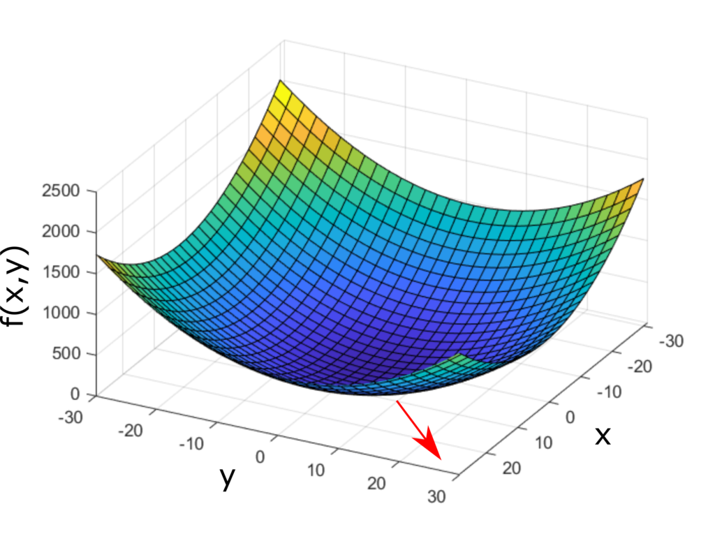
Figure 2: Gradient vector of the function (1) at the point $x=10$ and $y=10$ . The gradient is illustrated by the red arrow.

When the function $f$ depends on $n$ variables: $x_{1}$ , $x_{2}$ , …, $x_{n}$ , then the gradient is defined by

(5) $\begin{align*}g(x_{1},x_{2},\ldots,x_{n})=\nabla f(x_{1},x_{2},\ldots,x_{n})=\begin{bmatrix} \frac{\partial f}{\partial x_{1}} \\ \frac{\partial f}{\partial x_{2}}\\ \vdots \\ \frac{\partial f}{\partial x_{n}} \end{bmatrix}\end{align*}$

For presentation clarity, let us return to the example of the function of two variables. Everything explained in this tutorial can easily be generalized to the case of functions depending on three or more variables. Several important facts about this gradient should be observed:

The gradient is equal to zero at the point $(x=2,y=2)$ . This point is actually the minimum of the function. That is, the function achieves the minimum at the point $(x,y)$ for which the gradient is equal to zero. We have
(6) $\begin{align*}g(x,y)=\nabla f=\begin{bmatrix} 2(x-2) \\ 2(y-2) \end{bmatrix}=\begin{bmatrix} 0\\0 \end{bmatrix}\end{align*}$

This expression is zero for $x=2$ and $y=2$ , and from the form of the function (1), we conclude that the minimum is achieved at $x=2$ and $y=2$ .

On the other hand, if our function was for example

(7) $\begin{align*}q(x,y)=-(x-2)^{2}-(y-2)^{2}\end{align*}$

Then, the gradient is

(8) $\begin{align*}\nabla q(x,y)=\begin{bmatrix}-2(x-2) \\ -2(y-2) \end{bmatrix}\end{align*}$

The function $q(x,y)$ achieves a maximum at the point $(x=2,y=2)$ , that is, it achieves the maximum value at the point for which its gradient is equal to zero. These simple examples confirm that the candidate points for (local) minimum and maximum of functions are the points for which their gradients become equal to zero. Keep in mind that these are only necessary conditions for a local extremum. The sufficient conditions involve Hessians of functions. This topic is out of the scope of this tutorial.

The gradient is a vector whose value at a certain point is the direction and rate of the (locally) fastest increase of the function $f$ . For example, the gradient at the point $(x=10,y=10)$ of the function $f(x,y)$ defined by the equation (1) is

(9) $\begin{align*}g(10,10)=\begin{bmatrix} 16 \\ 16 \end{bmatrix}\end{align*}$

That is, the direction of the fastest increase is a vector

(10) $\begin{align*}\begin{bmatrix} 16 \\ 16 \end{bmatrix} =16 \begin{bmatrix} 1 \\ 1 \end{bmatrix}\end{align*}$

Let us numerically illustrate this fact. That is, let us show that starting at the point $(x=10,y=10)$ , the direction of the fastest increase of the function is positively collinear with the vector (10). Suppose that at the point $(x=10,y=10)$ , we move in the direction of a vector that is positively collinear with the gradient vector. We assume that we take a small step in this direction. We can select an infinite number of vectors that are collinear with the gradient vector. The most natural choice is the following unit vector:

(11) $\begin{align*}\begin{bmatrix} 0.7071 \\ 0.7071 \end{bmatrix}\end{align*}$

That is, new point $(x_{1},y_{1})$ at which we want to evaluate the value of the function $f$ is

(12) $\begin{align*}x_{1}=10+0.7071=10.7071,\; y_{1}=10+0.7071=10.7071\end{align*}$

The value of the function $f$ at this point is

(13) $\begin{align*}f(x_{1},y_{1})=(10.7071-2)^{2}+(10.7071-2)^{2}=151.6272\end{align*}$

Now, let us assume that at the point $(x=10,y=10)$ , we move in the direction of another unit vector, which makes an angle of 60 degrees with respect to the x-axis. Again, we assume that we take small steps in this direction. The vector is

(14) $\begin{align*}\begin{bmatrix} 1 \cos(60) \\ 1 \sin(60) \end{bmatrix}=\begin{bmatrix} 0.5 \\ 0.8660 \end{bmatrix}\end{align*}$

Let us evaluate the value of the function $f$ at a new point in the direction of this vector. The new point is defined by

(15) $\begin{align*}x_{2}=10+0.5=10.5,\; y_{2}=10+0.8660=10.8660\end{align*}$

The value of the function $f$ at this point is

(16) $\begin{align*}f(x_{2},y_{2})=(10.5-2)^{2}+(10.8660-2)^{2}=150.8560\end{align*}$

And obviously, this value is smaller than the value of the function at the point $(x_{1},y_{1})$ in the direction of the gradient vector. Similarly, it can be numerically verified that if we take any direction, along any unit vector from the point $(x=10,y=10)$ , except for the direction of the unit vector that is positively collinear with the gradient, and take a small step, we will always have a smaller function value than the value of the function in the direction of the unit vector positively collinear with the gradient vector.

To properly understand gradients, it is also important to introduce the concept of level curves for the case when the function $f$ depends on two variables and the concept of level surfaces for the case when the function $f$ depends on three or more variables. Consider the function $z=f(x,y)$ . The level curve of this function is defined by

(17) $\begin{align*}f(x,y)=c\end{align*}$

where $c$ is a constant. Obviously, the equation (17) defines a curve that is the intersection of the function $f(x,y)$ with the horizontal plane parallel to the xy plane with the distance of $c$ from the xy plane.

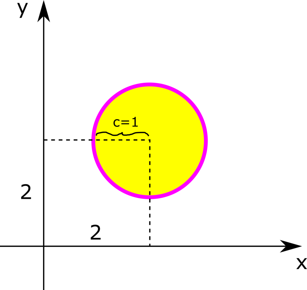
In the case of the function defined by (1) the level curves are obviously circles centered at $(2,2)$ with the radius of $\sqrt{c}$ :

(18) $\begin{align*}(x-2)^{2}+(y-2)^{2}=c\end{align*}$

The figure below illustrates the level curve.

Figure 3: Level curve of the function (1).

In the same manner, we can define the level surfaces for functions with three or more variables. For example, for the function

(19) $\begin{align*}f(x,y,z)=x^{2}+y^{2}+z^{2}\end{align*}$

The level surface is given by the following equation

(20) $\begin{align*}x^{2}+y^{2}+z^{2}=c\end{align*}$

Obviously, this is a sphere with the radius of $\sqrt{c}$ centered at zero.

Why are the level curves and level surfaces relevant to the concept of gradients?

Because of this reason:

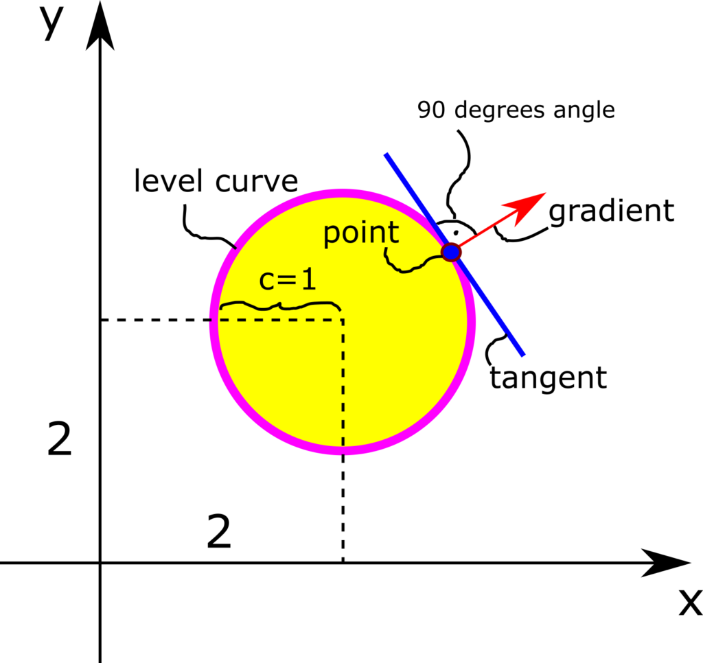
The gradient at point $(x,y)$ is perpendicular to the level curve (level surface) that passes through that point. More precisely, the gradient at the point $(x,y)$ is perpendicular to the tangent (the tangent plane in the case of level surfaces) of the level curve (level surface) at the point $(x,y)$ . This is illustrated in the figure below for the function (1) and for $c=1$ .

Figure 4: Level curves, gradients, and tangent lines.

Batch Gradient Descent Method

Now that we understand the concept of gradient, let us explain how this concept can be used to solve optimization problems in batch form. The name of this method is the batch gradient descent method which is also known as the steepest descent method and gradient descent method. The word “batch” refers to the data batch, that is, optimization problems in the batch form depend on a data batch:

(21) $\begin{align*}\begin{bmatrix}y_{1} \\ y_{2} \\ \vdots \\ y_{N}\end{bmatrix},\;\; \begin{bmatrix}x_{1} \\ x_{2} \\ \vdots \\ x_{N}\end{bmatrix}\end{align*}$

where $(x_{1},y_{1}),(x_{2},y_{2}),\ldots, (x_{N},y_{N})$ are data points. These data points represent the data batch.

Here, for presentation clarity, we assume that these data points are related through a linear model. However, everything explained in this tutorial can easily be generalized to nonlinear models. Let us assume that the data points are related through a linear model that we want to estimate

(22) $\begin{align*}y=\theta_{1}x+\theta_{2}\end{align*}$

where $\theta_{1}$ and $\theta_{2}$ are parameters of the linear model that we need to estimate. The previous equation is an ideal representation of a physical system or a process. For example, the model (22) can represent a calibration curve of our sensor. For example, $y$ might be a measured voltage, $x$ can a physical variable that we are interested in observing, such as distance, pressure, or temperature. The parameters $\theta_{1}$ and $\theta_{2}$ are unknown parameters of the model that need to be estimated. In practice, the model (22) is always corrupted by measurement noise.

The goal is to estimate the parameters $\theta_{1}$ and $\theta_{2}$ , from the set of batch data $(x_{1},y_{1}),(x_{2},y_{2}),\ldots, (x_{N},y_{N})$ .

By using the data points and from (22), we have

(23) $\begin{align*}y_{1}& =\theta_{1}x_{1}+\theta_{2}+n_{1}\\y_{2}& =\theta_{1}x_{2}+\theta_{2}+n_{2} \\& \vdots \\y_{N}&=\theta_{1}x_{N}+\theta_{2}+n_{N}\end{align*}$

where $n_{1},n_{2},\ldots, n_{N}$ represent measurement noise for every data point $(x_{i},y_{i})$ , $i=1,2,3,\ldots, N$ .

To estimate the parameters, we form the batch cost function:

(24) $\begin{align*}J(\theta_{1},\theta_{2})= \sum_{i=1}^{N} \big(y_{i}-\theta_{1}x_{i}-\theta_{2} \big)^{2}\end{align*}$

and we form the batch optimization problem

(25) $\begin{align*}\min_{\theta_{1},\theta_{2}} J(\theta_{1},\theta_{2}) = \min_{\theta_{1},\theta_{2}} \sum_{i=1}^{N} \big(y_{i}-\theta_{1}x_{i}-\theta_{2} \big)^{2}\end{align*}$

This optimization problem is a linear least-squares problem for which we can find the closed-form solution. This is explained in our previous post. However, in this tutorial, we will not use such a solution that is only applicable to linear least-squares problems. Instead, we will use the batch gradient descent (also known as the gradient descent method or the steepest descent method) that is applicable to a much more general class of optimization problems that also includes nonlinear optimization problems and nonlinear least squares problems.

The idea of the batch gradient descent is to approximate the solution of the optimization problem (25) iteratively. Let the optimization variables be grouped inside of the vector $\boldsymbol{\theta}$ , defined by

(26) $\begin{align*}\boldsymbol{\theta}=\begin{bmatrix} \theta_{1} \\ \theta_{2} \end{bmatrix}\end{align*}$

The batch gradient descent method approximates the solution by propagating this iteration

(27) $\begin{align*}\boldsymbol{\theta}^{(k+1)}=\boldsymbol{\theta}^{(k)}-\gamma \nabla J(\boldsymbol{\theta}^{(k)})\end{align*}$

where

The vector of optimization variables at the iteration $k$ is

(28) $\begin{align*}\boldsymbol{\theta}^{(k)}=\begin{bmatrix} \theta_{1}^{(k)} \\ \theta_{2}^{(k)} \end{bmatrix}\end{align*}$

$k$ is the index of the current iteration
$\gamma$ is the step size (learning rate). This is a relatively small real number either selected by the user or selected by using specialized methods, such as line search methods. Here, we assumed that this number is constant and independent from the index $k$ of the current iteration. However, this number can also depend on the current iteration.
The gradient of the cost function $J(\boldsymbol{\theta})$ evaluated at $\boldsymbol{\theta}^{(k)}$ is denoted by
(29) $\begin{align*}\nabla J(\boldsymbol{\theta}^{(k)})\end{align*}$

We propagate the batch gradient descent iteration (27) for $k=0,1,2,3,\ldots$ , until convergence of the cost function or optimization vector variables.

So, what is the physical motivation behind the batch gradient descent method (27)?

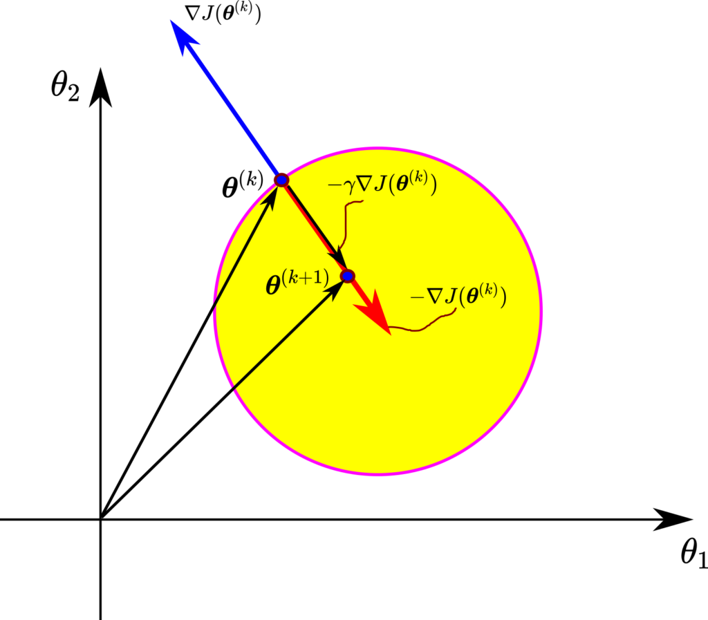
Consider the illustration shown after this paragraph. We learned that the gradient vector points to the direction of the fastest increase of a function and is essentially equal to the rate of the fastest increase of the function. Now, if we add a minus sign in front of the gradient, we obtain the opposite direction. In this opposite direction, the decrease of the function will be maximized. If we decrease the function value along this direction starting from the current value of the optimization variable vector $\boldsymbol{\theta}^{(k)}$ , we are doing a good job. That is, we should expect that the cost function will decrease if we move the optimization variable vector in this direction. However, we need to scale our step, so we multiply the negative gradient with a step size that is usually a small number. If we add this negative and scaled gradient to our vector $\boldsymbol{\theta}^{(k)}$ , we get the vector of optimization variables $\boldsymbol{\theta}^{(k+1)}$ . The cost function value at the vector $\boldsymbol{\theta}^{(k+1)}$ should be smaller than the cost function value at the optimization vector $\boldsymbol{\theta}^{(k)}$ . We repeat this procedure iteratively for $k=0,1,2,\ldots$ .

Figure 5: Graphical interpretation of the gradient descent method. The pink circle is the level curve of the cost function.

Let us compute the gradient of the cost function (24), so we can implement the batch gradient descent method in Python. The gradient vector is given by

(30) $\begin{align*}\nabla J(\boldsymbol{\theta})=\begin{bmatrix} \frac{\partial J}{\partial \theta_{1}} \\ \frac{\partial J}{\partial \theta_{2}} \end{bmatrix}=\begin{bmatrix} \sum_{i=1}^{N} 2\big(y_{i}-\theta_{1}x_{i}-\theta_{2} \big)(-x_{i}) \\ \sum_{i=1}^{N} 2\big(y_{i}-\theta_{1}x_{i}-\theta_{2} \big)(-1) \end{bmatrix}\end{align*}$

By introducing the error variable

(31) $\begin{align*}e_{i}=y_{i}-\theta_{1}x_{i}-\theta_{2} \end{align*}$

By substituting this definition in (30), we have

(32) $\begin{align*}\nabla J(\boldsymbol{\theta})=\begin{bmatrix} -2\sum_{i=1}^{N} e_{i}x_{i} \\ -2\sum_{i=1}^{N} e_{i} \end{bmatrix}\end{align*}$

Python Implementation of Batch Gradient Method

First, we import the necessary libraries and generate the data batch.

# -*- coding: utf-8 -*-
"""
Python implementation of the Batch gradient descent and stochastic gradient descent
"""
import numpy as np
import matplotlib.pyplot as plt

# generate the data

# true value of the parameters that we want to estimate
theta1true=2
theta2true=-2
xValues=np.linspace(-5,5,25)
yValues=np.zeros(xValues.shape)
for i in range(len(xValues)):
    # here, change the constant multiplying np.random.normal() to increase/decrease the measurement noise
    yValues[i]=theta1true*xValues[i]+theta2true+0.01*np.random.normal()

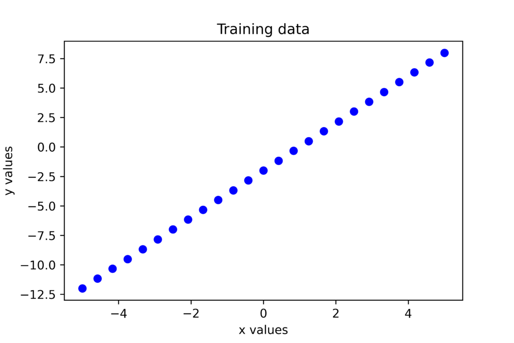
# plot the data set    
plt.plot(xValues,yValues,'bo')
plt.title('Training data')
plt.xlabel('x values')
plt.ylabel('y values')
plt.savefig('dataBatch.png',dpi=600)
plt.show()

We select the true value of the parameters $\theta_{1}=2$ and $\theta_{2}=-2$ .By using this code line:

yValues[i]=theta1truexValues[i]+theta2true+0.01np.random.normal()

We generate the vector “yValues”. Also, keep in mind that by adding the term “0.01np.random.normal()” we introduce the measurement noise. Initially, we assume a small value of noise in order to test the convergence of the method. The data that will be used for estimation is shown below.

Next, we define two functions. The first function will return a gradient of the cost function for the data-batch vectors “xValues” and “yValues” and for the current value of the optimization vector $\boldsymbol{\theta}$ . The second function will return the value of the cost function for the current value of the optimization vector and for the data-barch vectors. These functions are given below.

# this function returns the gradient of the cost function 
# formed for the data batch vectors x and y, and for the thetaParameterVector
# define the batch gradient function 
def gradientBatch(thetaParameterVector, x, y):
    gradientBatchValue=np.zeros(shape=(2,1))    
    gradientTheta1=0
    gradientTheta2=0
    for j in range(len(x)):
        error=(y[j]-thetaParameterVector[0]*x[j]-thetaParameterVector[1])
        gradientTheta1=gradientTheta1-2*error*x[j]
        gradientTheta2=gradientTheta2-2*error 
    
    gradientBatchValue[0]=gradientTheta1
    gradientBatchValue[1]=gradientTheta2
    
    return gradientBatchValue

# define the cost function for the current value of the optimization vector 
# and for the data batch vectors x and y
def costFunction(thetaParameterVector, x, y):
    costFunction=0
    for j in range(len(x)):
        costFunction=costFunction+(y[j]-thetaParameterVector[0]*x[j]-thetaParameterVector[1])**2
    return costFunction

Next, we select the number of iterations of the batch gradient descent method, the step size, and the initial guess of the optimization vector. Then, we define a for loop that implements the batch gradient descent method given by the equation (27). The code lines shown below perform these tasks

# batch gradient descent parameters 
# number of iterations
numberIterationsGradient=1000
# step size
stepSizeBatchGradient=0.0001
# initial value of the optimization variables 
thetaInitial=np.random.normal(size=(2,1))


# these list store the optimization parameters during iterations
theta1List=[]
theta2List=[]
# this list stores values of the cost function
costFunctionList=[]

# initialize the vector of optimization variables
thetaCurrent=thetaInitial
# here we iteratively update the vector of optimization variables 
for i in range(numberIterationsGradient):
    theta1List.append(thetaCurrent[0][0])
    theta2List.append(thetaCurrent[1][0])
    costFunctionList.append(costFunction(thetaCurrent,xValues,yValues))
    thetaNext=thetaCurrent-stepSizeBatchGradient*gradientBatch(thetaCurrent,xValues,yValues)
    thetaCurrent=thetaNext
    print(costFunctionList[i])

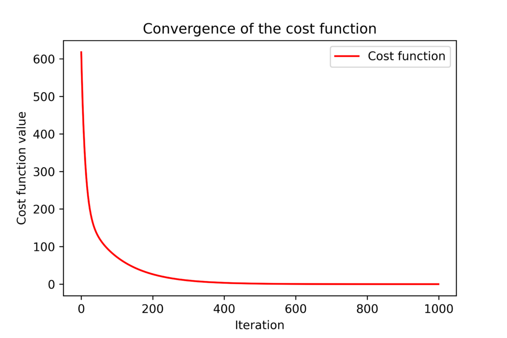
The batch gradient descent iteration is implemented in code line 23. We call the previously defined function “gradientBatch” which returns the value of the gradient at the current value of the optimization vector. We also update the list storing the current values of entries of the optimization vector and the current value of the cost function. This is important for investigating the convergence of the method. The figure below shows the convergence of the cost function $J(\boldsymbol{\theta}^{(k)})$ with respect to the optimization iteration index $k$ .

Figure 7: Convergence of the cost function (24) with respect to the optimization iteration index $k$ .

The figure below shows the convergence of the parameters $\theta_{1}$ and $\theta_{2}$ which are the entries of the optimization vector $\boldsymbol{\theta}$ .

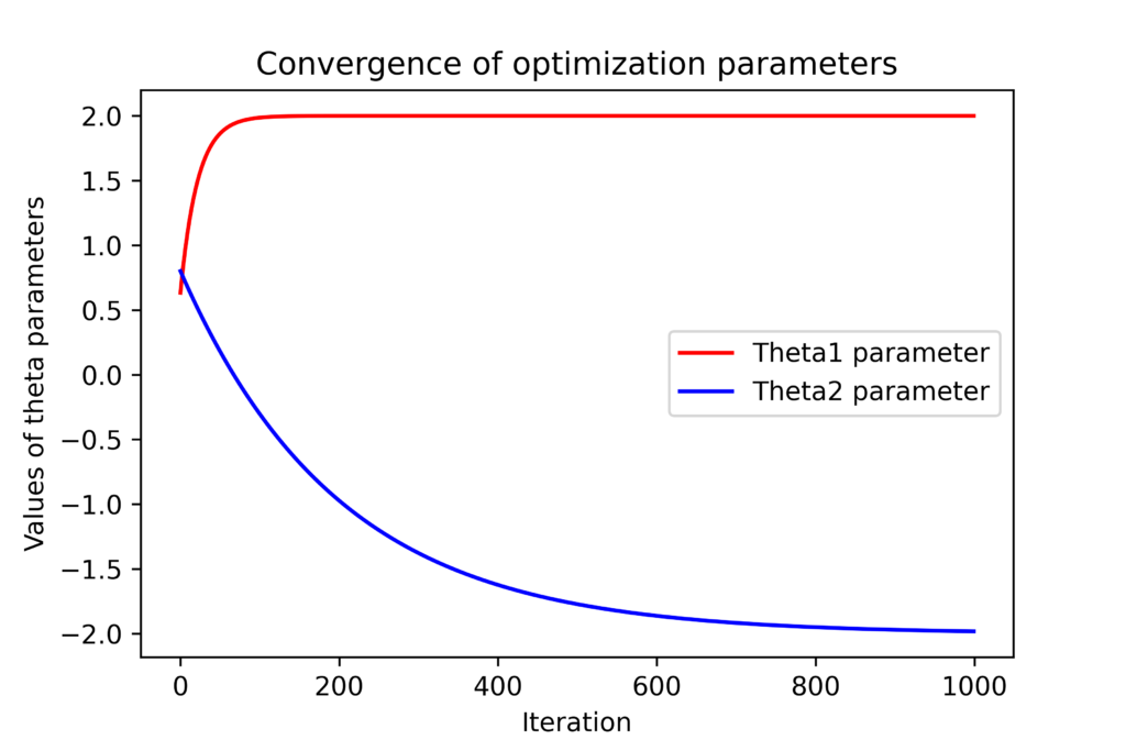Figure 8: convergence of the parameters $\theta_{1}$ and $\theta_{2}$ with respect to the optimization iteration index $k$ .4

We can observe that the entries of the optimization vector converge to the true values. However, they will never converge to the exact values due to the introduced measurement noise, unless we have an extremely large number of data samples. The figures shown above are generated by using these code lines.

plt.title('Convergence of the cost function')
plt.plot(costFunctionList,'r',label='Cost function')
plt.xlabel('Iteration')
plt.ylabel('Cost function value')
plt.legend()
plt.savefig('convergenceCostFunction.png',dpi=600)
plt.show()


plt.title('Convergence of optimization parameters')
plt.plot(theta1List,'r',label='Theta1 parameter')
plt.plot(theta2List,'b',label='Theta2 parameter')
plt.xlabel('Iteration')
plt.ylabel('Values of theta parameters')
plt.legend()
plt.savefig('convergenceTheta.png',dpi=600)
plt.show()

What is a Gradient?

Batch Gradient Descent Method

Python Implementation of Batch Gradient Method

admin

You might also like

Explanation and Python Implementation of On-Policy SARSA Temporal Difference Learning – Reinforcement Learning Tutorial with OpenAI Gym

Compute and Simulate Linear Quadratic Regulator (LQR) in MATLAB for Set Point Tracking

Tutorial on How to Create URDF File and Model of 4-Wheeled Mobile Robot in ROS