Clear Explanation of Breadth-First Graph Traversal and Breadth-First Search Algorithms with Python Implementation

In this computer science and robotics tutorial, we explain one very important algorithm that serves as the basis of a number of algorithms in computer science and robotics. In the context of graph traversal, the name of the algorithm is the breadth-first graph traversal algorithm. On the other hand, in the context of the graph search algorithms, the name of this algorithm is the breadth-first search algorithm. Essentially, it is the same algorithm only used for two applications. The understanding of this algorithm is important for developing more complex algorithms for graph problems in computer science, machine learning, and robotics. The YouTube video accompanying this tutorial is given below.

Basics of Queue Data Structure

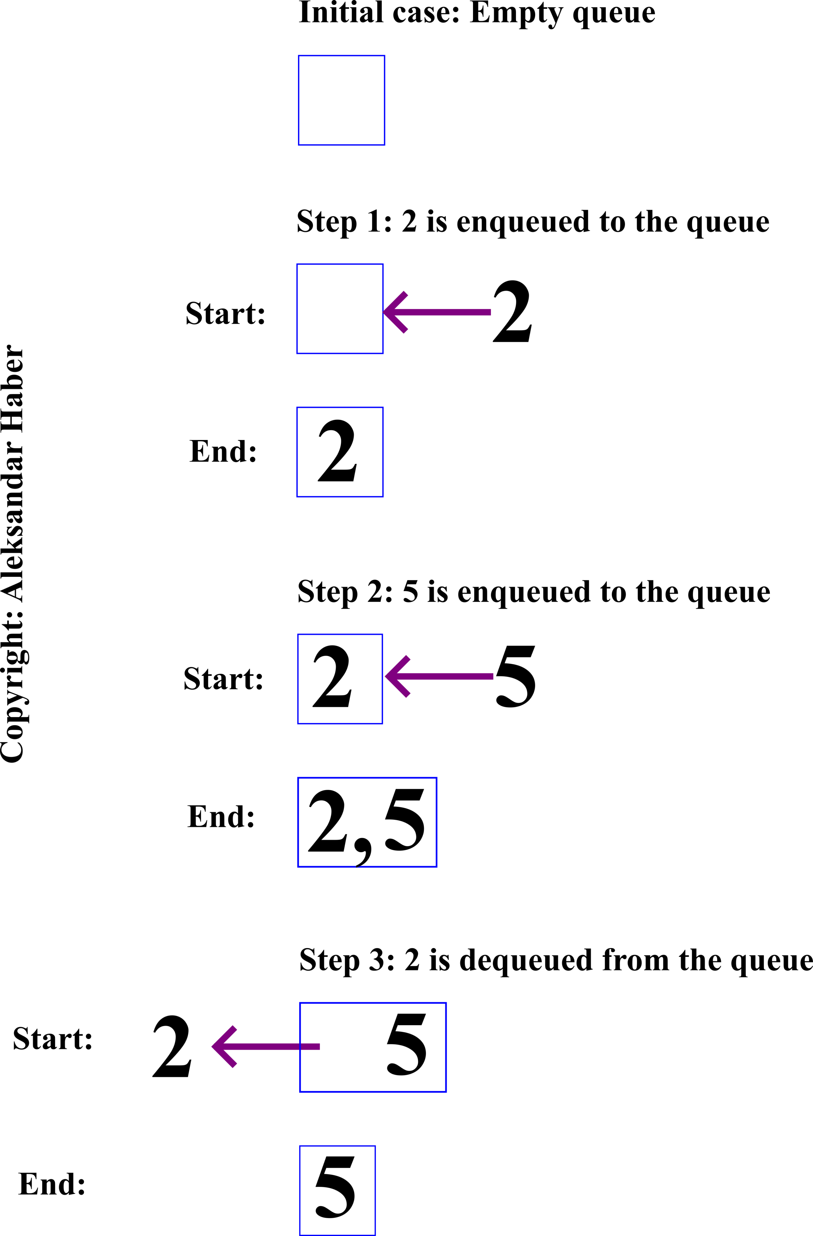
In order to properly understand the breadth-first search and graph traversal algorithm, we need to understand the queue data structure. This data structure implements the First-In-First-Out (FIFO) data containers. That is, the queue is a container that stores data elements by using the first-in-first-out data storage and retrieval principle.

In the context of queue data structures, the verb “enqueue” means to add or insert an item to the queue. The item is inserted at the end of the queue. On the other hand, the verb “dequeue” means to remove or eliminate an item from the queue. The item that is at the beginning of the queue is removed. Let us illustrate this with a graphical example.

Breadth-First Graph Traversal Algorithm

To explain the breadth-first graph traversal algorithm, we will consider the graph example given below.

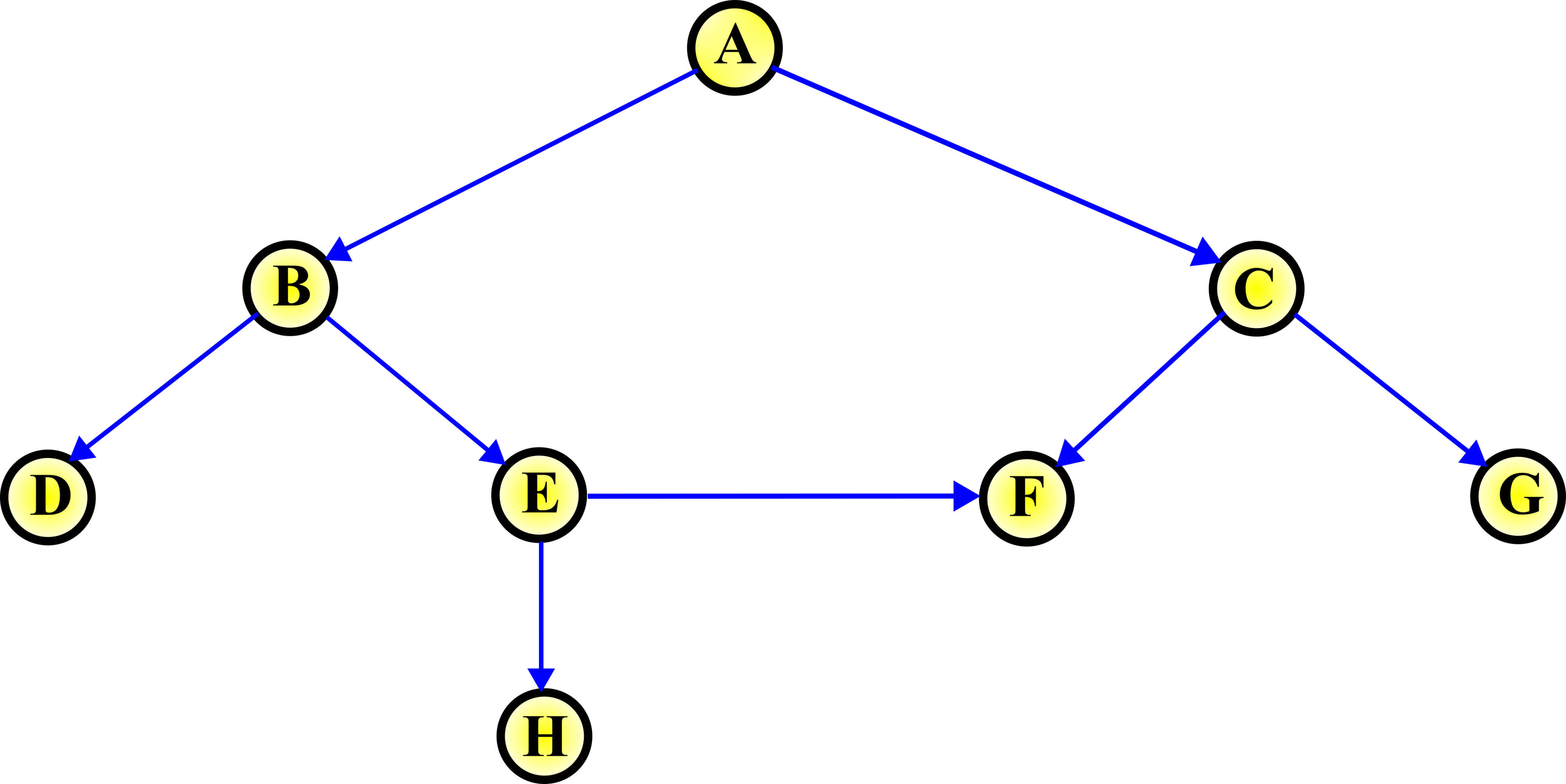
Graph Traversal Problem: Consider the graph shown in Fig. 2. above. Design an algorithm that will visit every node (vertex) of the graph.

The breadth-first graph traversal algorithm is used to solve this problem. The breadth-first graph algorithm solves this problem by using the following idea. First, we start from the root node. In our case, the root node is the node A. Then, we visit all the nodes that are depth 1 (or distance 1) from the root node. In our case, these are the nodes B and C. Then, we visit all the nodes that are depth 1 (or distance 1) from the B node. In our case, they are D and E. Then, we repeat the same process for the node C. This produces the nodes F and G. We repeat this process until we visit all the nodes.

Before we start with more detailed explanations, we need to explain the meaning of the word “breadth”. The word “breadth” is the measure of how broad or wide an object is. The word “width” can also be used as a synonym. For example, we can say that “The breadth of the hallway is 10 meters”.

To implement the algorithm, we need to define a list and a queue.

1. We need to define a container that will store all the visited nodes. We will use a list to store the visited nodes. New explored nodes will always be compared with the list of visited nodes, and only if they are not in the list, they are added to the list. We call this list as “visited”.
2. We need to define a queue that will store nodes that are adjacent to the nodes that are encountered during our search, and whose adjacent nodes will be explored in the next iteration. We call this queue simply as “queue”.

We graphically explain the breadth-first graph algorithm.

INITIAL STEP

The initial step is shown in the graph below.

In the first step, we add the root node A to the visited list and queue.

STEP 1:

This step is graphically explained in the figure below.

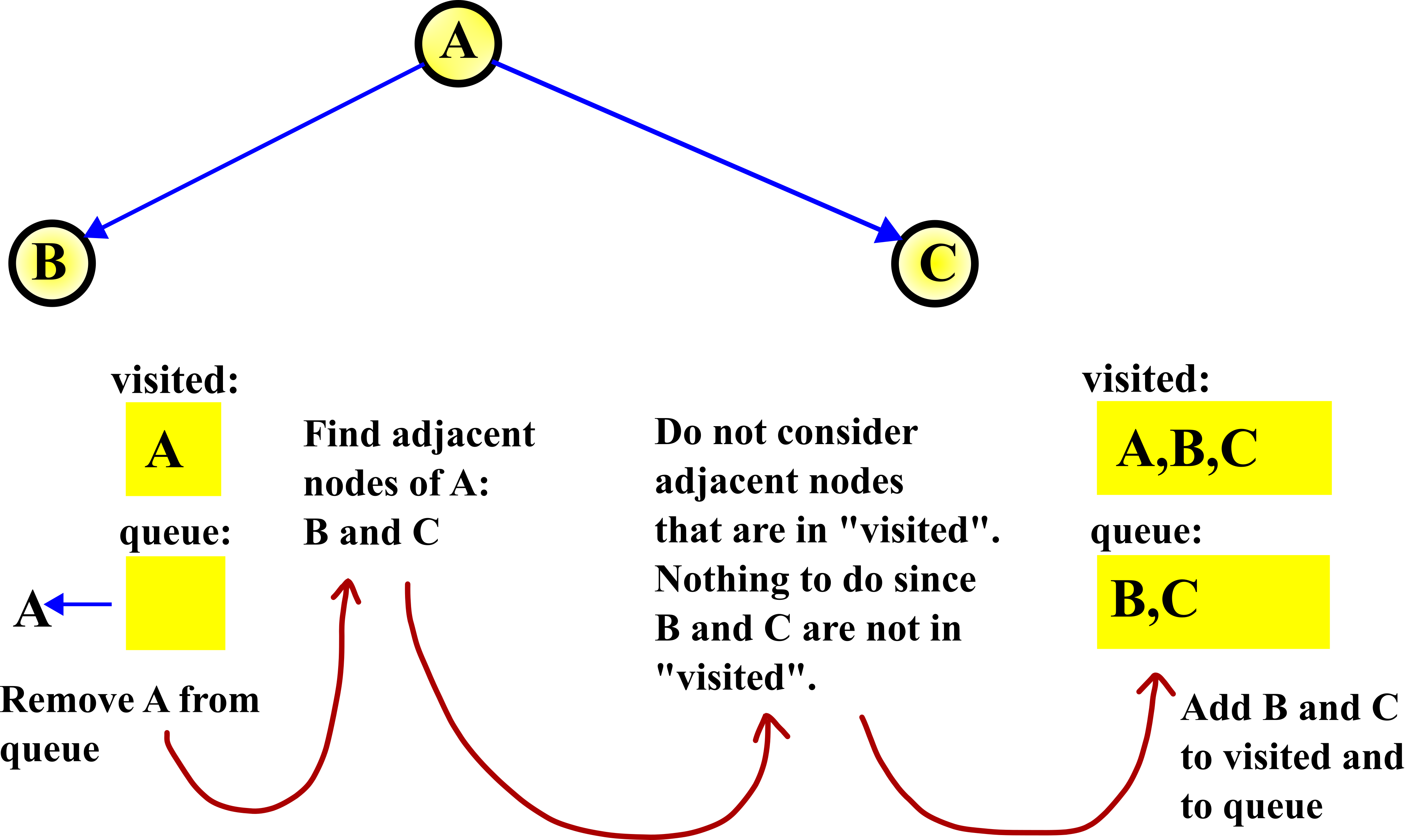
First, we remove A from the queue. That is, we select A. Then, we search for the adjacent nodes of the node A. These nodes are B and C. After that, we double-check if the nodes B and C are in the visited node list. They are not, and consequently, we add them to the visited node list. Then, we also add B and C to the queue, since their adjacent nodes need to be explored in the next step.

STEP 2:

The second step is illustrated in the figure below.

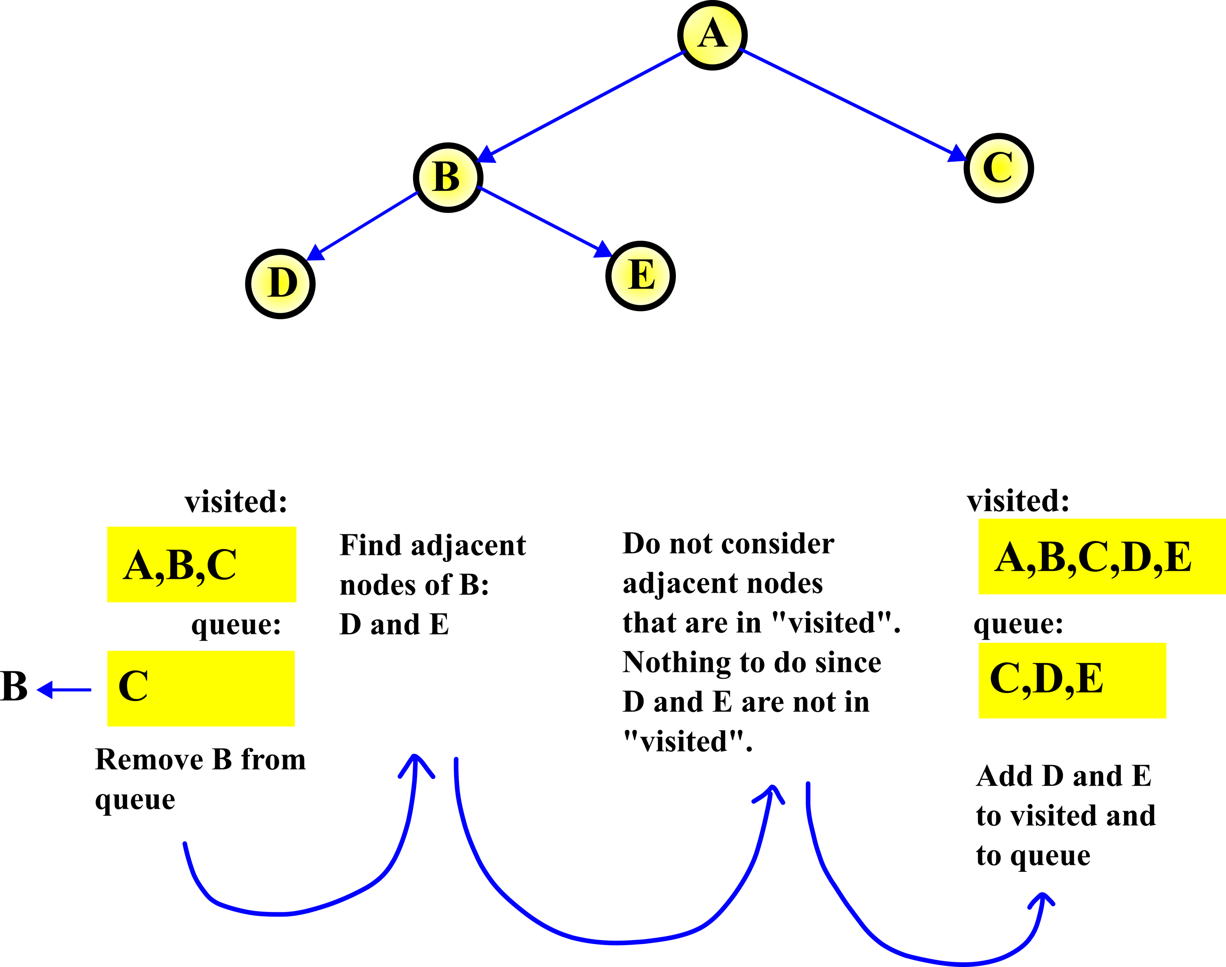
In the second step, we repeat the procedure from the first step. First, we remove B from the queue. That is, we select B, and then we explore (find) adjacent nodes of B. They are D and E. These nodes are not in the visited list, and consequently, we add them to this list. Also, we add them to the queue, since their potential adjacent nodes need to be explored.

STEP 3:

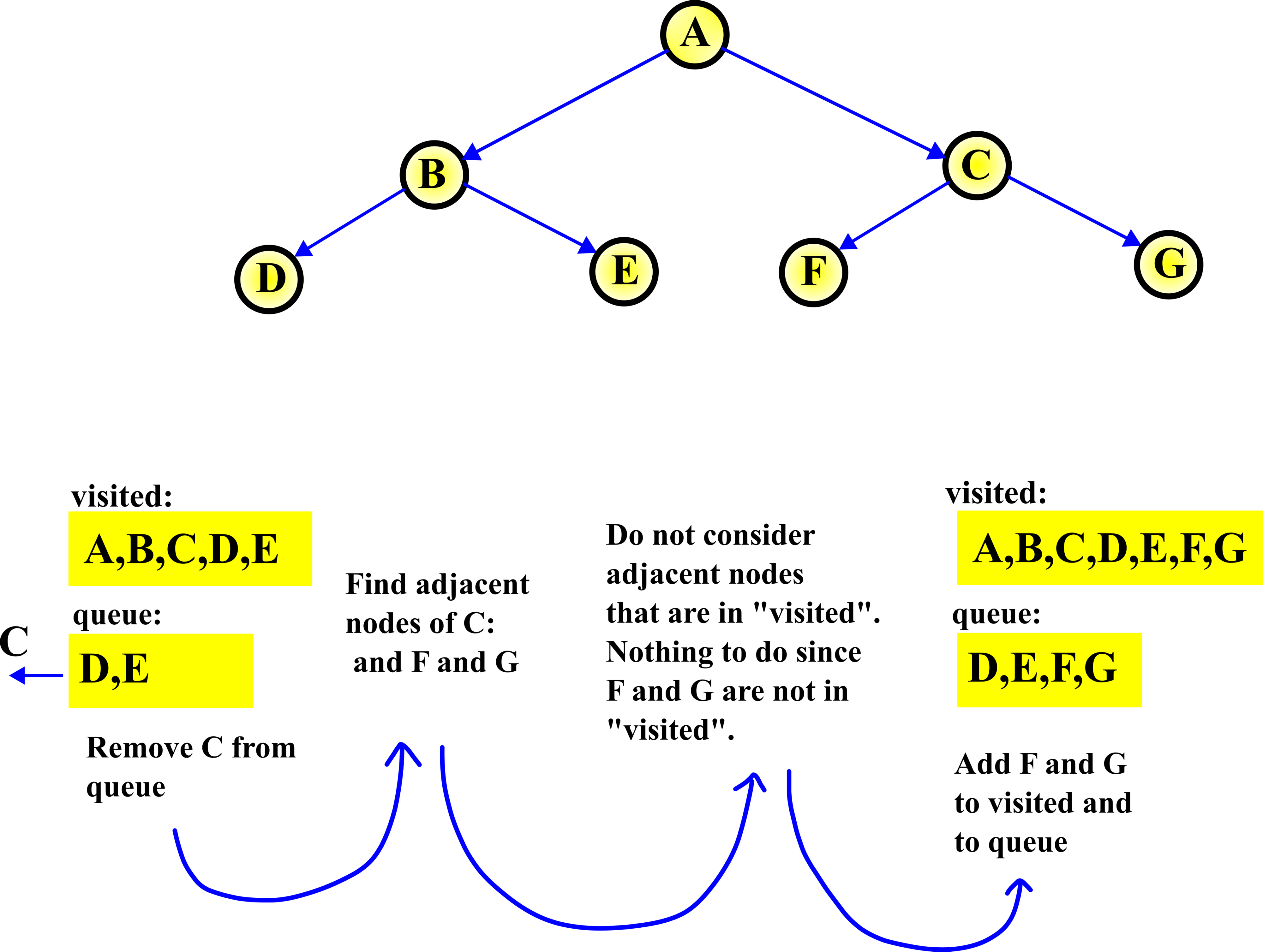
In the third step, we repeat the procedure from the second step. First, we remove C from the queue. That is, we select C, and then we explore (find) adjacent nodes of C. They are F and G. These nodes are not in the visited list, and consequently, we add them to this list. Also, we add them to the queue, since their potential adjacent nodes need to be explored.

With this step, we completed the first and second-level depth search. That is, we found all the nodes that are distance 1 and 2 from the root node.

STEP 4:

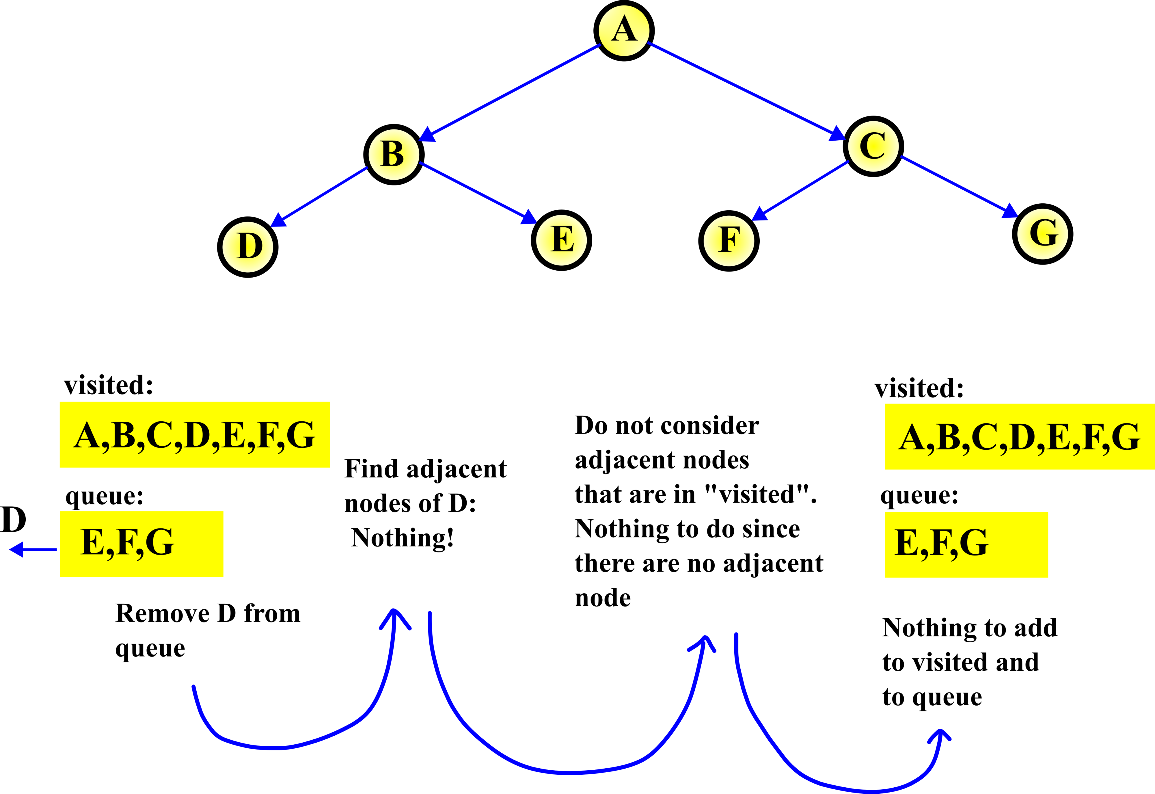
In the fourth step, we repeat the procedure from the third step. First, we remove D from the queue. That is, we select D, and then we explore (find) adjacent nodes of D. There are no adjacent nodes of D. Then, we do not need to add anything to the visited list and to the queue.

STEP 5:

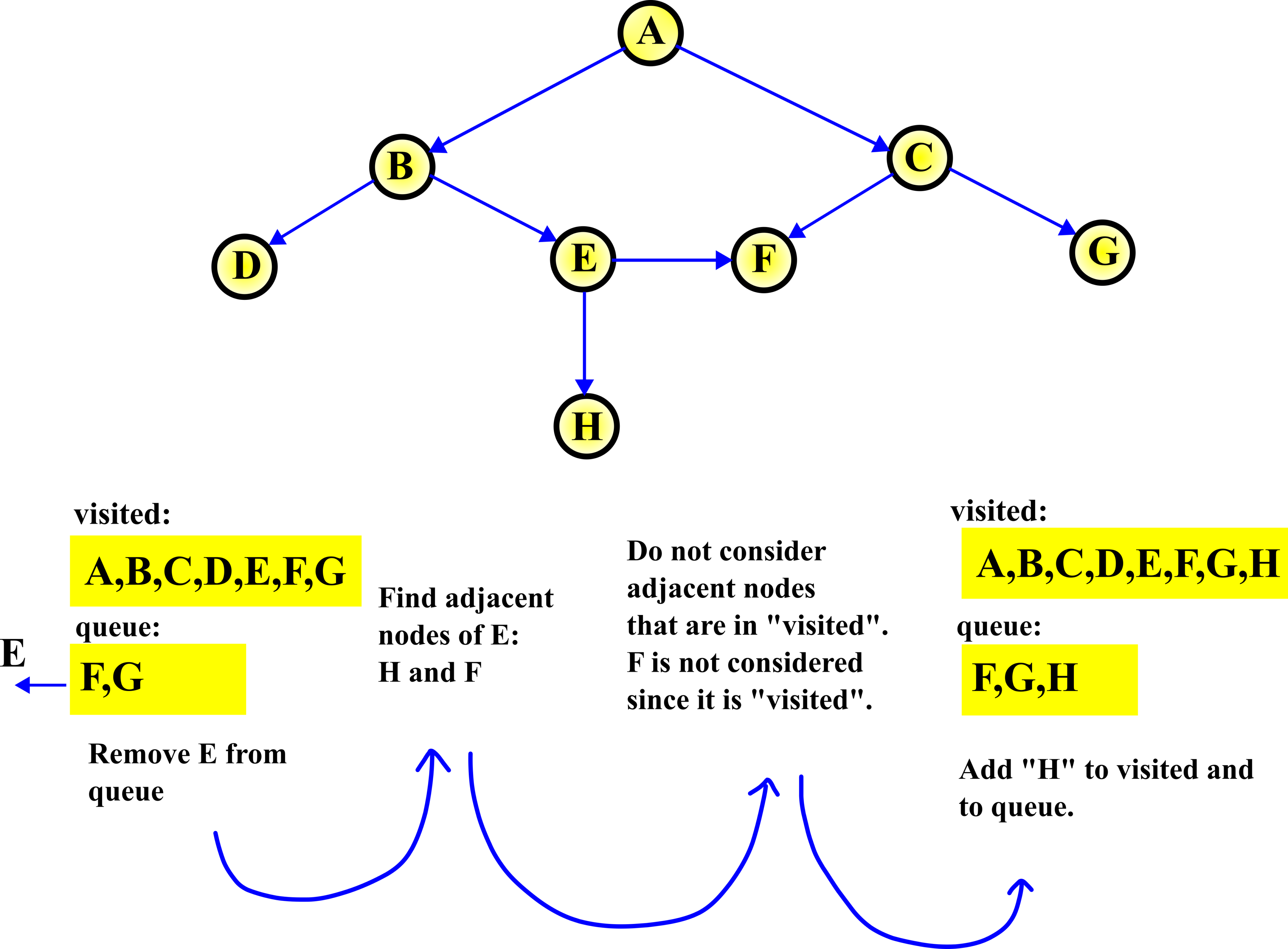
In the fifth step, we repeat the procedure from the fourth step. First, we remove E from the queue. That is, we select E, and then we explore (find) adjacent nodes of E. There are two adjacent nodes of E: H and F. Here, we do not consider F since it is already in the visited list. Consequently, we only need to add H to the visited list and to the queue.

STEP 6:

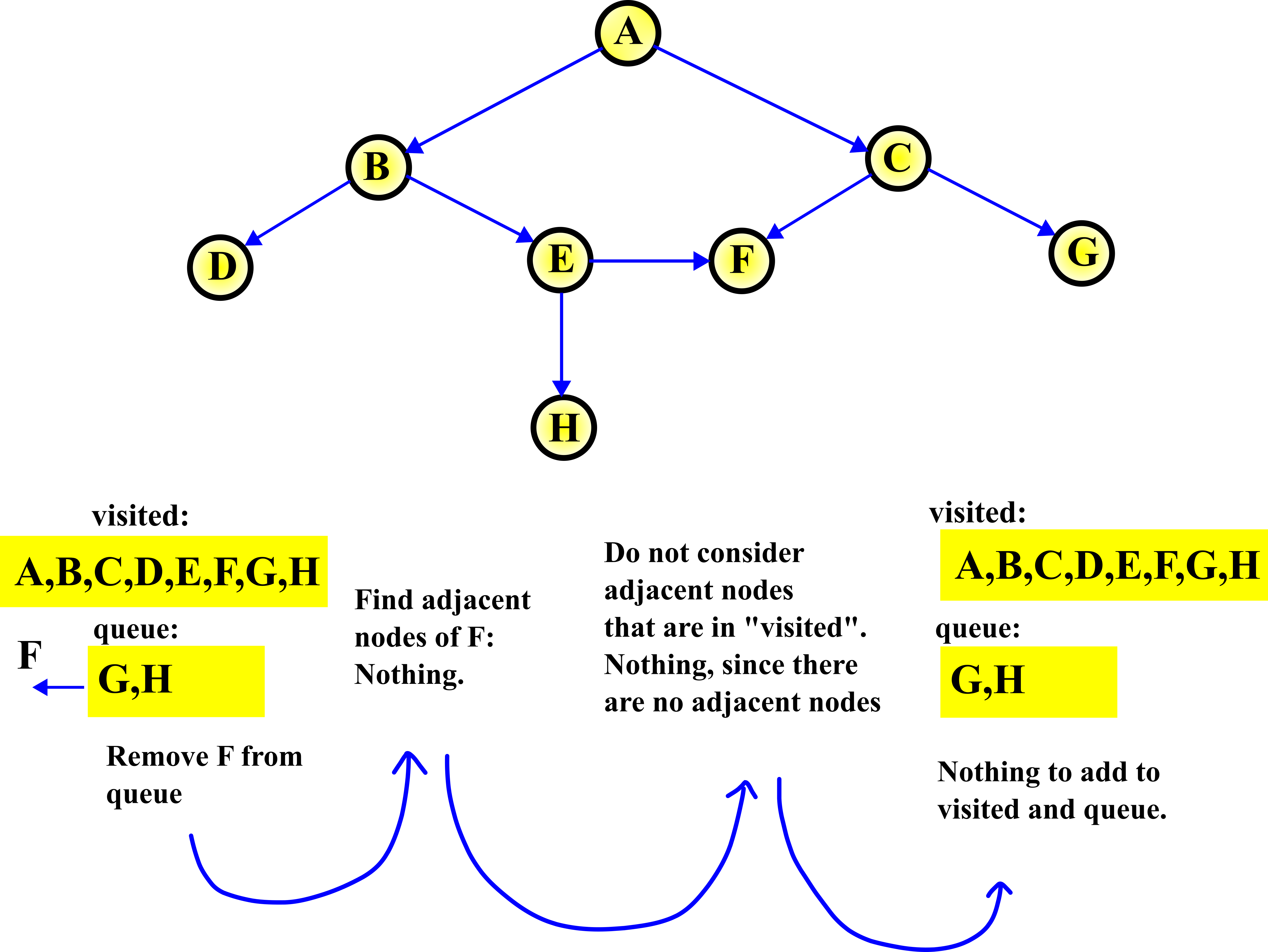
In this step, we remove F from the queue. Then, since there are no adjacent nodes of F, there is nothing to do.

STEP 7:

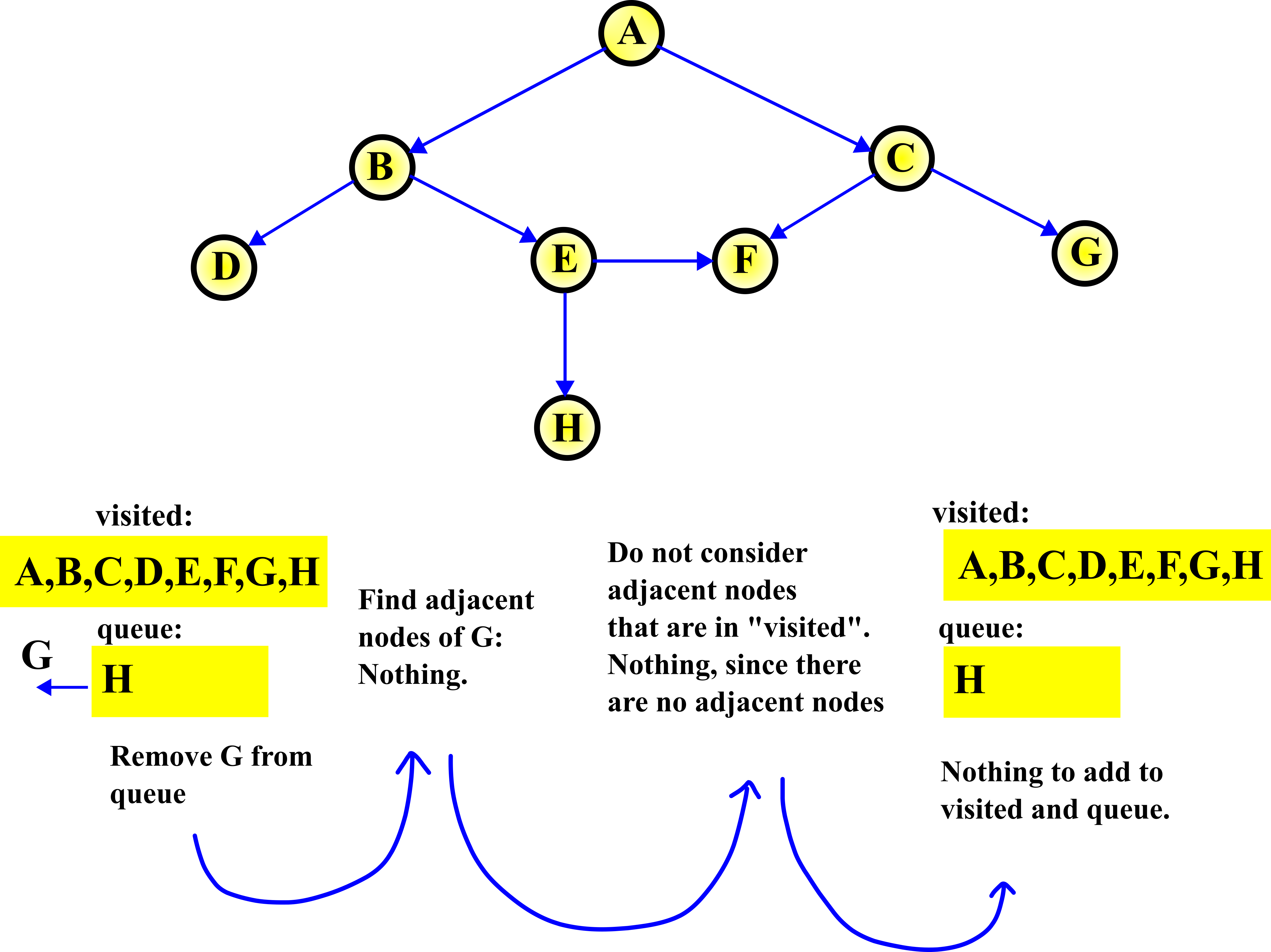
In this step, we remove G from the queue. Then, since there are no adjacent nodes of G, there is nothing to do.

STEP 8:

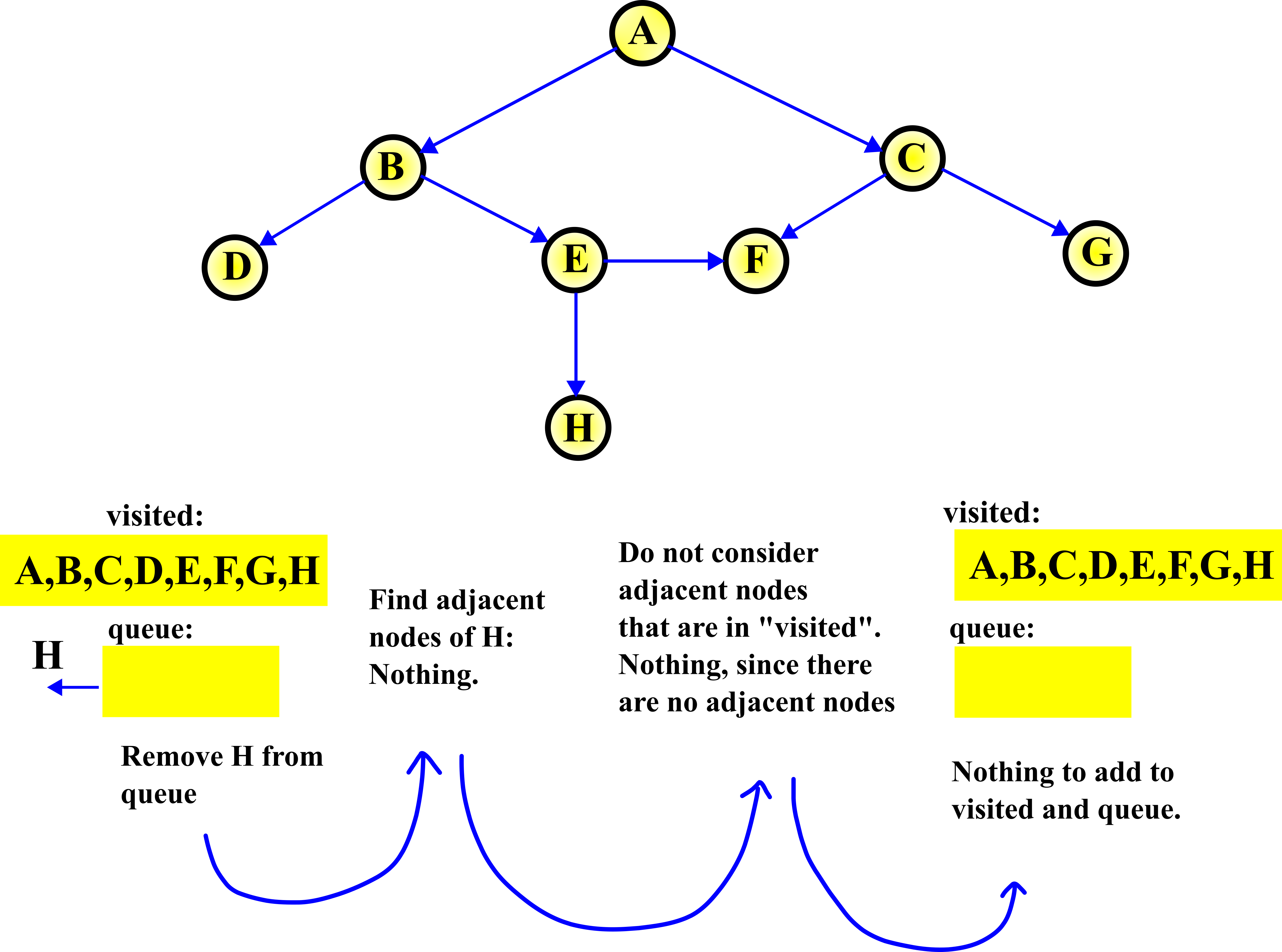
In this step, we remove H from the queue. Then, since there are no adjacent nodes of H, there is nothing to do.

This completes the graph traversal. We visited all the nodes in the graph.

Breadth-First Search Algorithm

The breadth-first search algorithm uses the same principle as the breadth-first graph traversal algorithm. We only formulate the problem and explain how the breadth-first graph traversal algorithm should be modified such that it can be used in the breadth-first search algorithm.

Graph search problem: Consider the graph shown in Fig. 12. above. Design an algorithm that will find a particular node. For example, node E.

We use the graph traversal algorithm, and we stop when we find the required node.

Python implementation of the Breadth-First Traversal Algorithm

First, we define the graph by using a Python dictionary:

# -*- coding: utf-8 -*-
"""
Demonstration of Breadth-First Graph Traversal Algorithm in Python
Author: Aleksandar Haber
November 2023

"""
# we use deque for queue
from collections import deque

# First, we create the adjacency list of our graph 
# we use dictionaries to crate graphs in Python
graphDict=dict()
graphDict['A']=['B','C']
graphDict['B']=['D','E']
graphDict['C']=['F','G']
graphDict['D']=[]
graphDict['E']=['H','F']
graphDict['F']=[]
graphDict['G']=[]
graphDict['H']=[]

Then, we implement the breadth-first graph traversal algorithm:

# this list is used to store visited nodes
visited=['A']
queue = deque(['A'])

# run this while the queue is non-empty
while (len(queue)>0):
    # dequeue (extract) the node from the queue
    currentNode=queue.popleft()
    # this is the list of nodes that are adjacent to the current node 
    listAdjacentNodesToCurrent=graphDict[currentNode]
    # if nodes are in the visited list, exclude them
    listAdjacentNodesToCurrentNotVisited=[a for a in listAdjacentNodesToCurrent if a not in visited] 
    # sort the node names according to the alphabetic order
    listAdjacentNodesToCurrentNotVisited =sorted(listAdjacentNodesToCurrentNotVisited)
    if (len(listAdjacentNodesToCurrentNotVisited)>0):
        for entry in listAdjacentNodesToCurrentNotVisited:
            visited.append(entry)
            queue.append(entry)

print(visited)

The above script will produce:

['A', 'B', 'C', 'D', 'E', 'F', 'G', 'H']