Tutorial on Simple Position Controller for Differential Drive Robot (Mobile Robot) with Simulation and 2D Animation in Python – Fusion of Engineering, Control, Coding, Machine Learning, and Science

In this control engineering and robotics tutorial, we explain the basics of position controllers for mobile robots. As a test case, we use a differential drive robot. Differential drive robots are also called differential wheeled robots. We design a simple proportional controller that will drive the robot center from the initial to the desired location. We use a kinematics robot model developed in our previous tutorial to simulate the robot’s motion. We explain how to generate a 2D Pygame animation that simulates the robot’s motion and control performance. Here, it should be kept in mind that we develop a controller that is based on the kinematics of the robot without taking into account the robot’s dynamics described by mass, moments of inertia, and dynamics equations. The Python scripts used to implement the control algorithm and to simulate robot motion are available here.

The YouTube tutorial accompanying this post is given below.

Differential Drive Robot Position Controller

Here, we first briefly summarize the kinematics diagram and the kinematics differential equation model of the robot. For details, see our previous tutorial given here. The robot kinematic diagram is shown below.

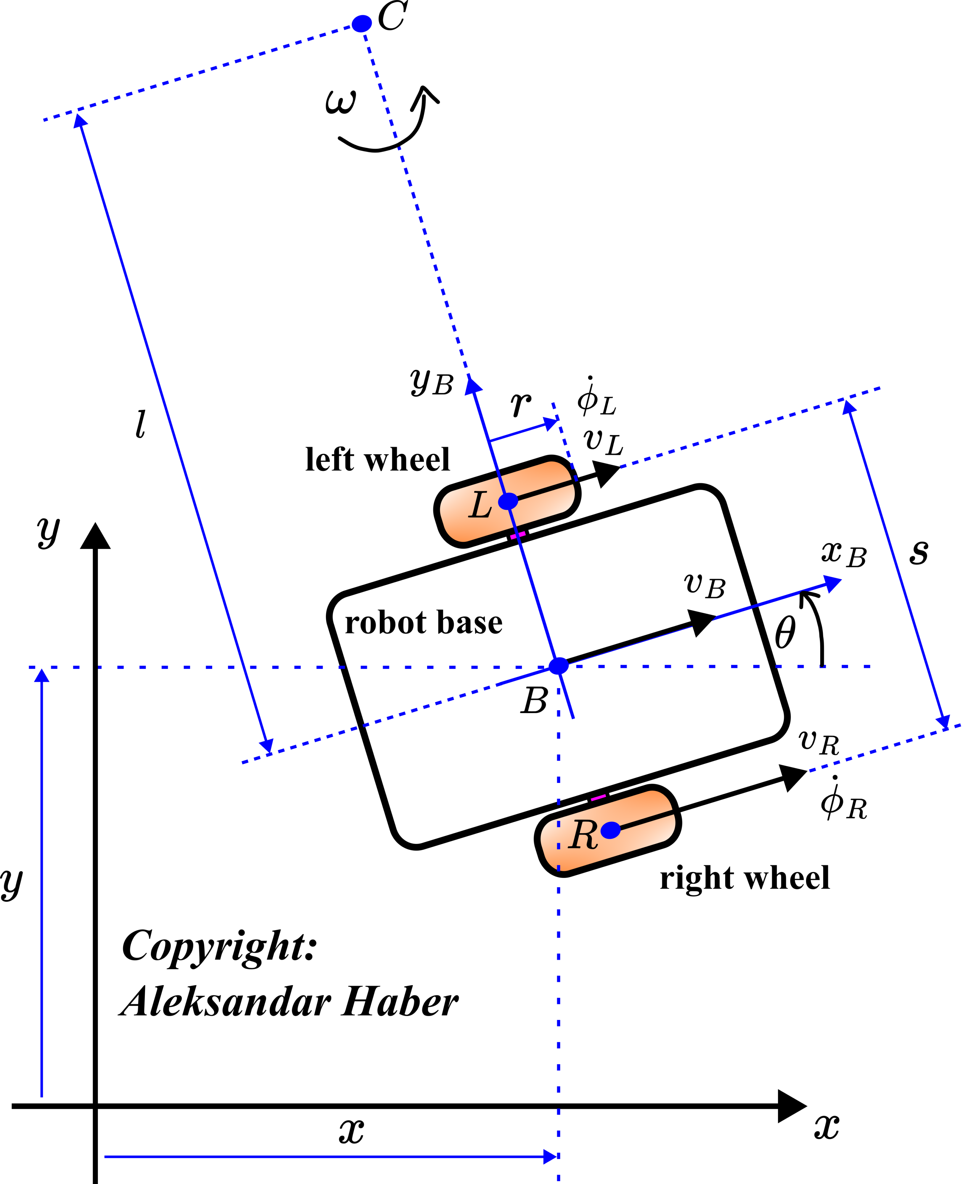
Figure 1: Kinematic diagram of the differential drive robot.

The symbols used in this figure are explained below.

$x$ and $y$ are the translation coordinates of the body frame attached to the point $B$ with respect to the inertial frame $x-y$ .
$\theta$ is the angle of rotation of the robot which is at the same time the angle between the body frame and the inertial frame.
$x_{B}$ and $y_{B}$ are the coordinates in the body frame and at the same time they denote the axes of the body frame.
$C$ is the instantaneous center of rotation.
$\omega$ is the instantaneous angular velocity of the robot body.
$L$ is the center point of the left wheel.
$R$ is the center point of the right wheel.
$B$ is the middle point between the points $L$ and $R$ .
$v_{L}$ is the velocity of the center of the left wheel.
$v_{R}$ is the velocity of the center of the right wheel.
$v_{B}$ is the velocity of the point $B$ .
$\dot{\phi}_{L}$ is the angular velocity of the left wheel.
$\dot{\phi}_{R}$ is the angular velocity of the right wheel.
$l$ is the distance between the point $B$ and the point $C$ .
$r$ is the radius of the wheels.
$s$ is the distance between the points $L$ and $R$ .
$\dot{x}$ is the projection of the velocity $v_{B}$ on the $x$ axis.
$\dot{y}$ is the projection of the velocity $v_{B}$ on the $y$ axis.

The kinematics system of differential equations describing the robot motion is given below (for more details, see our previous tutorial, given here):

(1) $\begin{align*}\dot{x}& =\frac{r\dot{\phi}_{L}}{2}\cos(\theta) +\frac{r\dot{\phi}_{R}}{2}\cos(\theta) \\\dot{y}& =\frac{r\dot{\phi}_{L}}{2}\sin(\theta) +\frac{r\dot{\phi}_{R}}{2}\sin(\theta) \\\dot{\theta} & = -\frac{r}{s}\dot{\phi}_{L}+ \frac{r}{s}\dot{\phi}_{R}\end{align*}$

On the other hand, for the implementation of the control algorithm, we need another equation relating $v_{B}$ and $\dot{theta}$ with $\dot{\phi}_{L}$ and $\dot{\phi}_{R}$ . This equation is given below:

(2) $\begin{align*}\begin{bmatrix} v_{B} \\ \dot{\theta} \end{bmatrix}= \begin{bmatrix} \frac{r}{2} & \frac{r}{2} \\ -\frac{r}{s} & \frac{r}{s} \end{bmatrix}\begin{bmatrix} \dot{\phi}_{L} \\ \dot{\phi}_{R}\end{bmatrix}\end{align*}$

The robot is controlled by controlling the left and right wheel angular velocities represented by $\dot{\phi}_{L}$ and $\dot{\phi}_{R}$ , respectively. For given values of $\dot{\phi}_{L}$ and $\dot{\phi}_{R}$ we can determine the robot position $(x,y)$ and orientation $\theta$ by integrating the system of equations (1).

In this tutorial, we are mainly interested in driving the center of the robot $B$ to a desired (target or reference) location, without controlling the orientation $\theta$ . That is, the robot can have an arbitrary orientation in the desired location. The control problem can be formally described as follows.

Control Problem Formulation: Let $x_{D}$ and $y_{D}$ be the $x$ and $y$ coordinates of the desired (target or reference) location of the robot center $B$ . Determine a sequence of wheel angular velocity control variables $\dot{\phi}_{L}$ and $\dot{\phi}_{R}$ such that the current robot position $(x(t),y(t))$ is equal to the desired robot position $(x_{D},y_{D})$ . Here, we assume that at any time instant, we can precisely measure the robot position $(x(t),y(t))$ and the robot orientation angle $\theta(t)$ .

There are a number of approaches to solving this problem. Since this is an introductory tutorial, we will use a relatively simple approach based on a proportional controller. Here, the interested reader should keep in mind that this is NOT the most optimal controller that will optimize the travel distance, used energy, or a similar quantity.

The following diagram is instrumental in deriving the control algorithm

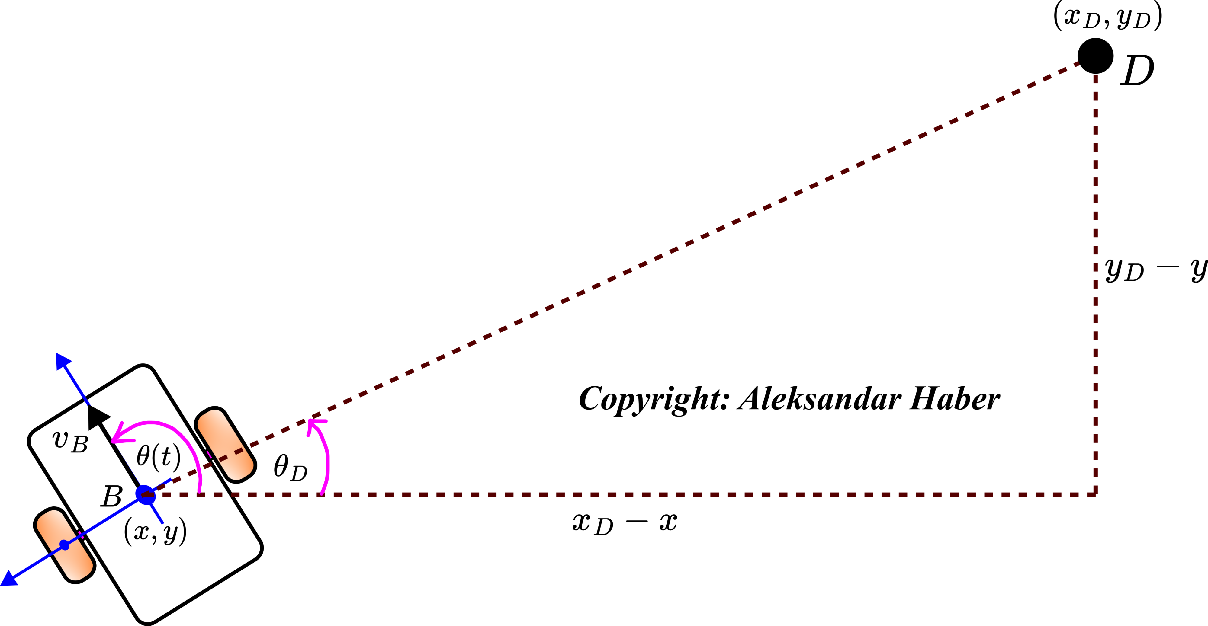
Figure 2: Illustration of the robot control problem

Let us suppose that at some time instant $t$ , the robot position is given by the coordinates $x$ and $y$ . Also, let us assume that at the time instant $t$ , the orientation of the robot body is given by $\theta(t)$ . Our goal is to steer the robot to the point $D$ with the coordinates $(x_{D},y_{D})$ . We assume that the robot’s center has the velocity $v_{B}(t)$ .

Here, one important geometrical observation should be made. The velocity vector $v_{B}(t)$ is tangent to the robot’s trajectory. Also, during a small time interval, this is the direction of the motion of the robot. To arrive at the target, we want to rotate this velocity vector such that it is in the direction of the line connecting the points $B$ and $D$ . That is, the angle $\theta$ should be equal to the angle $\theta_{D}$ of the line connecting the points $B$ and $D$ . By rotating the robot in this direction, we will achieve that the velocity is in the direction of the line connecting $B$ and $D$ .

From the current robot’s position, we can calculate the desired orientation angle $\theta_{D}$ as follows

(3) $\begin{align*}\tan (\theta_{D})=\frac{y_{D}-y}{x_{D}-x}\end{align*}$

(4) $\begin{align*}\theta_{D}=\arctan2 \Big( \frac{y_{D}-y}{x_{D}-x}\Big) \end{align*}$

where the $\arctan 2()$ (or $atan2()$ ) is the modified $\arctan ()$ or the 2-argument arctangent function that takes into account the signs of the arguments when computing the angles.

The first controller is the controller that will change $\theta$ . We use the proportional controller that has the following form

(5) $\begin{align*}\dot{\theta}=K_{\theta}\big( \theta_{D} -\theta(t)\big)\end{align*}$

where $\theta(t)$ is the current value of the orientation of the robot and $K_{\theta}$ is the proportional control gain for orientation control.

What is the physical meaning of the equation (5)? If the $\theta_{D} = \theta(t)$ , then according to this equation $\dot{\theta}=0$ and there is no change of $\theta$ since we have achieved the desired robot orientation.

The orientation controller actually controls the angle of the velocity. However, we need a controller that will control the magnitude of the velocity. This controller will implicitly also control the position of the robot. The second controller has the following form

(6) $\begin{align*}v_{B}=K_{v}\sqrt{(x_{D}-x(t))^{2}+(y_{D}-y(t))^{2}}\end{align*}$

where $K_{v}$ is the proportional constant for controlling the robot’s velocity. This controller will change the intensity of the velocity. However, it will not change the direction of the velocity. The direction of the velocity vector is changed by the orientation controller (5). This controller penalizes the Euclidean distance between the point $B$ and the point $D$ . The larger the distance is, the larger the magnitude of the velocity $v_{B}$ . As we get closer and closer to the desired location $D$ , the intensity of the velocity $D$ gradually decreases.

The controllers (5) and (6) determine the values of $\dot{\theta}$ and $v_{B}$ . However, we need to control the angular velocities of the wheels $\dot{\phi}_{L}$ and $\dot{\phi}_{R}$ . To control these angular velocities, we need to transform $\dot{\theta}$ and $v_{B}$ into $\dot{\phi}_{L}$ and $\dot{\phi}_{R}$ . We can do that by inverting the system of equations (2). Namely, from this equation, we can express $\dot{\phi}_{L}$ and $\dot{\phi}_{R}$ as follows

(7) $\begin{align*}\begin{bmatrix} \dot{\phi}_{L} \\ \dot{\phi}_{R}\end{bmatrix} = \begin{bmatrix} \frac{r}{2} & \frac{r}{2} \\ -\frac{r}{s} & \frac{r}{s} \end{bmatrix}^{-1} \begin{bmatrix} v_{B} \\ \dot{\theta} \end{bmatrix}\end{align*}$

That is, we invert the parameter matrix

(8) $\begin{align*}\begin{bmatrix} \frac{r}{2} & \frac{r}{2} \\ -\frac{r}{s} & \frac{r}{s} \end{bmatrix}\end{align*}$

Now, we are ready to summarize the control algorithm.

Summary of Control Algorithm for Differential Drive Robot

The control algorithm consists of the following steps.

We observe the robot position $x(t),y(t)$ and the robot orientation $\theta(t)$
We compute
(9) $\begin{align*}\dot{\theta} & =K_{\theta}\big( \theta_{D} -\theta(t)\big) \\v_{B} &=K_{v}\sqrt{(x_{D}-x(t))^{2}+(y_{D}-y(t))^{2}}\end{align*}$
We compute the desired angular wheel velocities $\dot{\phi}_{L}$ and $\dot{\phi}_{R}$ as follows
(10) $\begin{align*}\begin{bmatrix} \dot{\phi}_{L} \\ \dot{\phi}_{R}\end{bmatrix} = \begin{bmatrix} \frac{r}{2} & \frac{r}{2} \\ -\frac{r}{s} & \frac{r}{s} \end{bmatrix}^{-1} \begin{bmatrix} v_{B} \\ \dot{\theta} \end{bmatrix}\end{align*}$
Apply the computed values $\dot{\phi}_{L}$ and $\dot{\phi}_{R}$ to the left and right wheel motor controllers that will generate the torques and move the wheels of the differential drive robot.

As mentioned at the beginning of this tutorial, we are not considering the dynamics of the robot. For us, the complete robot model is described by the kinematics equations (1). We are aware that this is an approximation, however, for robots with small masses and small moments of inertia this approximation can be sufficiently accurate to design the control inputs. Consequently, in our simulation, the model (1) serves as the “true” physical model of the robot. Over here, we write again these equations for clarity:

(11) $\begin{align*}\dot{x}& =\frac{r\dot{\phi}_{L}}{2}\cos(\theta) +\frac{r\dot{\phi}_{R}}{2}\cos(\theta) \\\dot{y}& =\frac{r\dot{\phi}_{L}}{2}\sin(\theta) +\frac{r\dot{\phi}_{R}}{2}\sin(\theta) \\\dot{\theta} & = -\frac{r}{s}\dot{\phi}_{L}+ \frac{r}{s}\dot{\phi}_{R}\end{align*}$

That is, in our simulations, once we compute $\dot{\phi}_{L}$ and $\dot{\phi}_{R}$ , we will use these quantities in the equation (11) as the known inputs. In our simulations, we integrate the system of equations (11) to compute the values of $x(t),y(t)$ and the robot orientation $\theta(t)$ , and then we use these values in the step 1 of the control algorithm.

Python Simulation and Animation of Controller for Differential Drive Robot

We have developed Python codes for implementing the controller and for simulating the robot’s motion. We used Pygame to simulate the robot’s motion. The animations are shown in the video below. The Python scripts used to implement the control algorithm and to simulate robot motion are available here.

Differential Drive Robot Position Controller

Summary of Control Algorithm for Differential Drive Robot

Python Simulation and Animation of Controller for Differential Drive Robot

admin

You might also like

Quadratic Forms, Positive Definite, Negative Definite, and Semi-Definite Matrices

Model Predictive Control (MPC) Tutorial 1: Unconstrained Formulation, Derivation, and Implementation in Python from Scratch

Definition and Simulation of State-Space Models of Linear Systems in Python by Using Control Systems Library