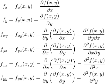
Calculate Minimum and Maximum Values of Functions of Two Variables – Fusion of Engineering, Control, Coding, Machine Learning, and Science

In this mathematics, engineering, and calculus tutorial, we explain how to calculate the minimum and maximum values of functions of two variables. This tutorial is important for a number of real-life engineering and physics problems. The YouTube tutorial accompanying this tutorial is given below. First, we briefly summarize theoretical results, and then, we give several examples at the end of this tutorial.

Theoretical Background

We consider a real-valued function $f(x,y)$ of two real variables $x$ and $y$ . Examples of these functions are given below

(1) $\begin{align*}f(x,y)& =x^{2}+y^{2}, \\f(x,y)& =\cos(x)\cdot\sin(x) \\f(x,y)& =2x_{1}^{2}+x_{1}x_{2}+\sin(x_{1})\end{align*}$

We want to determine (local) minimal and maximal values of such functions.

We assume that the function $f(x,y)$ is differentiable. Next, let us introduce the following abbreviated notation:

(2) $\begin{align*}f_{x} & =f_{x} (x,y)=\frac{\partial f(x,y)}{\partial x} \\f_{y} & =f_{y} (x,y)=\frac{\partial f(x,y)}{\partial y}\\f_{xy}& =f_{xy} (x,y)=\frac{\partial }{\partial y}\Big(\frac{\partial f(x,y)}{\partial x }\Big) = \frac{\partial^{2} f(x,y)}{\partial y \partial x} \\ f_{yx}& =f_{yx} (x,y)=\frac{\partial }{\partial x}\Big(\frac{\partial f(x,y)}{\partial y }\Big) = \frac{\partial^{2} f(x,y)}{\partial x \partial y} \\f_{xx}& =f_{xx} (x,y)=\frac{\partial }{\partial x}\Big(\frac{\partial f(x,y)}{\partial x }\Big) = \frac{\partial^{2} f(x,y)}{\partial^{2} x } \\f_{yy}& =f_{yy} (x,y)=\frac{\partial }{\partial y}\Big(\frac{\partial f(x,y)}{\partial y }\Big) = \frac{\partial^{2} f(x,y)}{\partial^{2} y }\end{align*}$

First, we state the following theorem

THEOREM 1 (CRITICAL POINTS AND EXTREME VALUES): If the function $f(x,y)$ has a (local) minimum or a (local) maximum at the point $x=a$ and $y=b$ , then

(3) $\begin{align*}f_{x}(a,b)=0 \\f_{y}(a,b)=0\end{align*}$

That is, if the function has a minimum or maximum at the point $(x=a,y=b)$ , then the partial derivatives $f_{x}$ and $f_{y}$ evaluated at these points are equal to zero!

The point $(a,b)$ is called the critical point or the stationary point if the following two conditions are satisfied:

(4) $\begin{align*}f_{x}(a,b)=0 \\f_{y}(a,b)=0\end{align*}$

Here it should be kept in mind that not all critical points produce minimum or maximum. One example is a saddle point. We will explain this later on when we do several examples. The next theorem gives us conditions for (local) minimum or maximum.

THEOREM 2(SECOND ORDER TEST): Let us suppose that the point $(a,b)$ is the critical point of the function $f(x,y)$ . Define the matrix P of partial derivatives as follows:

(5) $\begin{align*}P(x,y)=\begin{bmatrix} f_{xx} & f_{xy} \\ f_{yx} & f_{yy} \end{bmatrix}\end{align*}$

where $f_{xx}$ , $f_{xy}$ , $f_{yx}$ and $f_{yy}$ are defined in (2). Then, let the determinant of $P$ be defined by

(6) $\begin{align*}\text{det}(P(x,y))=f_{xx}f_{yy} - f_{yx} f_{xy} =f_{xx}f_{yy} - f_{xy}^{2}\end{align*}$

where we used the fact that $f_{xy}=f_{yx}$ . Let $\text{det}(P(a,b))$ be the value of the determinant of $P$ evaluated at the critical point $(a,b)$ . Then,

If $\text{det}(P(a,b))>0$ and $f_{xx}(a,b)>0$ , then the function $f(x,y)$ has a local minimum at the critical point $(a,b)$ .
If $\text{det}(P(a,b))>0$ and $f_{xx}(a,b)<0$ , then the function $f(x,y)$ has a local maximum at the critical point $(a,b)$ .
If $\text{det}(P(a,b))<0$ , then the function $f(x,y)$ does not have a local minimum at the critical point $(a,b)$ and the function $f(x,y)$ does not have a local maximum at the critical point $(a,b)$ . The point $(a,b)$ is then called the saddle point of the function $f(x,y)$ .

Here, it is very important to emphasize that if $\text{det}(P(a,b))=0$ , then we cannot conclude anything about minimum, maximum, or saddle point. In fact, the function can have a minimum/maximum value or a saddle point. However, we cannot conclude anything about the precise nature of this point.

Theoretical Background

admin

You might also like

Clear and Concise Explanation of the Law of Sines With Solved Examples

Control Systems Lecture: Basic Principles of Feedback Control

Multi-armed Bandit Problem: Epsilon-Greedy Action Value Methods With Python Codes and Implementation