Using Recurrent Neural Networks and Keras/TensorFlow to Learn Input-Output Behaviour of Dynamical Systems – Fusion of Engineering, Control, Coding, Machine Learning, and Science

This post was published on May 05, 2020. Please do not copy and paste this post in your blogs/posts/papers/reports. I am preparing a technical report that is based on this report, and I will post it online, so you can cite it if you plan to use some ideas from this post.

Before we start (for inpatient): the codes used in this project are posted here. The video accompanying this post is given below.

1. Motivation

This post is motivated by an interesting question posted on the Keras Github page.
The post starts with the following sentence: “For a final thesis I am working with Keras on Tensorflow and have to investigate how LSTM Networks can be used to identify dynamical systems.”

Feedforward neural networks have been extensively used for system identification of nonlinear dynamical systems and state-space models. However, it is interesting to investigate the potential of Recurrent Neural Network (RNN) architectures implemented in Keras/TensorFlow for the identification of state-space models. In this post, I present numerical experiments obtained by using Keras RNN architectures for learning the input-output behavior of dynamical systems. We explain the used Python codes, present conclusions, and give some recommendations. The codes can be found here.

2. Problem Formulation

So let us start with a problem definition. For presentation simplicity, we are going to give a problem formulation assuming a linear system. However, everything we explain straightforwardly applies to nonlinear systems. Various dynamical systems, such as robotic arms, oscillators, and even economic systems, can be mathematically described by a linearized state-space model having the following form:

(1) $\begin{align*}& \dot{\mathbf{x}}(t)=A\mathbf{x}(t)+B\mathbf{u}(t) \\& \mathbf{y}(t)=C\mathbf{x}(t)+ D\mathbf{u}(t) \notag\end{align*}$

where $t$ is time, $\mathbf{x}\in \mathbb{R}^{n}$ is the state vector, $\mathbf{u}\in \mathbb{R}^{m}$ is the input vector, and $\mathbf{y}\in \mathbb{R}^{r}$ is an output vector.
The matrices $A\in \mathbb{R}^{n\times n}$ , $B\in \mathbb{R}^{n\times m}$ , $\mathbf{C}\in \mathbb{R}^{r \times n}$ and $D\in \mathbb{R}^{r\times m}$ are the system matrices.
The vector $\mathbf{u}$ represents control inputs acting on the system. The vector $\mathbf{y}$ is the vector of observed variables, and the vector $\mathbf{x}$ is a state vector. Loosely speaking, this vector represents the internal system memory.

From a practical point of view, it is easier to estimate a discrete-time version of the original system. The discrete-time system has the following form:

(2) $\begin{align*}& \mathbf{x}_{k+1}=A\mathbf{x}_{k}+B\mathbf{u}_{k} \\& \mathbf{y}_{k}=C\mathbf{x}_{k}+ D\mathbf{u}_{k}\notag\end{align*}$

where $k$ is a discrete-time instant. That is, the state and other vectors are approximations of the original state at the time $t=kT$ , where $T$ is a sampling period.

The standard identification problem for the system (2) can be formulated as follows. Given the sequence of the input-output data $\{ \big(\mathbf{u}_{0}),\mathbf{y}_{0}\big), \big(\mathbf{u}_{1},\mathbf{y}_{1}\big), \ldots, \big(\mathbf{u}_{N},\mathbf{y}_{N}\big) \}$ , where $N$ is the length of the sequence, estimate the system matrices $A$ , $B$ , $C$ , and $D$ up to (unknown) similarity transformation. The estimated state-space model should accurately reproduce the input-output behavior of the original system.

Generally speaking, the recurrent neural network architectures such as Simple Recurrent Networks (SNR) or Long Short-Term Memory (LSTM) networks do not have the exact structure of the state-space model in (2). They might have the linear state-space model structure only in some special cases. For example, SNRs have the following representation:

(3) $\begin{align*}\mathbf{q}_{k}& =\boldsymbol{\sigma}_{q}\Big(L\mathbf{q}_{k-1}+E\mathbf{p}_{k}+\mathbf{z} \Big) \\\mathbf{v}_{k}&=\boldsymbol{\sigma}_{v}\Big(P\mathbf{q}_{k}+\mathbf{g} \Big) \end{align*}$

where $\mathbf{q}_{k}$ is a hidden layer vector, $\mathbf{p}_{k}$ is a Neural Network (NN) input vector, $\mathbf{v}_{k}$ is an NN output vector, $\mathbf{z}$ and $\mathbf{g}$ are vectors of NN parameters, $L,E$ and $P$ are matrices consisting of NN parameters, and $\boldsymbol{\sigma}_{q},\boldsymbol{\sigma}_{v}$ are vector activation function, and $k$ is discrete time.
Obviously, when activation functions are linear, and the parameter vectors $\mathbf{z}$ and $\mathbf{g}$ are zero, the SRN model (3) resembles the state-space model (2). So in some sense, the classical linear state-space model can be seen as an SNR and vice-versa.

Consequently, our goal is to train (learn) the parameters of recurrent neural networks such that trained networks produce the input-output behavior of the discrete-time state-space model (2).

That is, when we apply the sequence of control inputs $\{\mathbf{u}_{0},\mathbf{u}_{1},\ldots, \mathbf{u}_{N} \}$ (and an initial state of the system) to the neural network, it should produce the sequence of outputs $\{\hat{\mathbf{y}}_{0},\hat{\mathbf{y}}_{1},\ldots, \hat{\mathbf{y}}_{N} \}$ that accurately approximates the output sequence $\{\mathbf{y}_{0},\mathbf{y}_{1},\ldots, \mathbf{y}_{N} \}$ of the real-system.

In the sequel, we show how to perform this using the Keras/TensorFlow machine learning toolbox. For presentation clarity, this will be explained using an example of a mass-spring system.

3. Numerical Example and Python Codes

The mass-spring system is shown in Fig. 1. below.

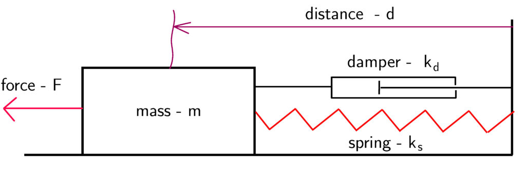
Figure 1: Mass-spring system used in numerical simulations.

The mathematical model is given by the following ordinary differential equation:

(4) $\begin{align*}m\ddot{d}+k_{d}\dot{d}+k_{s}d=F\end{align*}$

where $d$ is a distance from the equilibrium point, $m$ is the mass, $k_{d}$ and $k_{s}$ are damping and spring constants and $F$ is an external force.
By introducing the state-space variables $x^{(1)}=d$ and $x^{(2)}=\dot{d}$ , the model (4) can be written in the state-space form

(5) $\begin{align*}\underbrace{\begin{bmatrix}\dot{x}^{(1)} \\ \dot{x}^{(2)}\end{bmatrix}}_{\dot{\mathbf{x}}}= \underbrace{\begin{bmatrix} 0 & 1 \\ -\frac{k{s}}{m} & -\frac{k_{d}}{m}\end{bmatrix}}_{A} \underbrace{\begin{bmatrix} x^{(1)} \\ x^{(2)}\end{bmatrix}}_{\mathbf{x}}+\underbrace{\begin{bmatrix} 0 \\ \frac{1}{m} \end{bmatrix}}_{B}\underbrace{F}_{\mathbf{u}} \end{align*}$

We assume that only the position vector $d$ (that is, the state variable $x^{1}$ ) can be observed. Consequently, the output equation takes the following form:

(6) $\begin{align*}\mathbf{y}=\underbrace{\begin{bmatrix}1 & 0\end{bmatrix}}_{C}\mathbf{x} \end{align*}$

The state-space model (5)-(6) of the spring-mass system is in the continuous-time domain. To transform it into the discrete-time domain we use the Backward Euler method. Using this approximation, we obtain:

(7) $\begin{align*} \frac{\mathbf{x}_{k}-\mathbf{x}_{k-1}}{h}=A\mathbf{x}_{k}+B\mathbf{u}_{k-1}\end{align*}$

where $h$ is the discretization time step. The last equation leads to

(8) $\begin{align*}\mathbf{x}_{k}=\tilde{A}\mathbf{x}_{k-1}+\tilde{B}\mathbf{u}_{k-1} \end{align*}$

where $\tilde{A}=(I-hA)^{-1}$ and $\tilde{B}=h\tilde{A}B$ , and the output equation remains unchanged:

(9) $\begin{align*} \mathbf{y}_{k}=C\mathbf{x}_{k} \end{align*}$

Next, we present a Python code for computing the system response on the basis of the backward Euler method. The code will be used to generate training, validation, and test data for recurrent neural networks.

import numpy as np
import matplotlib.pyplot as plt

# define the continuous-time system matrices

A=np.matrix([[0, 1],[- 0.1, -0.05]])
B=np.matrix([[0],[1]])
C=np.matrix([[1, 0]])
#define an initial state for simulation
x0=np.random.rand(2,1)

#define the number of time-samples used for the simulation and the sampling time for the discretization
time=300
sampling=0.5

#define an input sequence for the simulation
#input_seq=np.random.rand(time,1)
input_seq=np.ones(time)
#plt.plot(input_sequence)


# the following function simulates the state-space model using the backward Euler method
# the input parameters are:
#    -- A,B,C              - continuous time system matrices 
#    -- initial_state      - the initial state of the system 
#    -- time_steps         - the total number of simulation time steps 
#    -- sampling_perios    - the sampling period for the backward Euler discretization 
# this function returns the state sequence and the output sequence
# they are stored in the vectors Xd and Yd respectively
def simulate(A,B,C,initial_state,input_sequence, time_steps,sampling_period):
    from numpy.linalg import inv
    I=np.identity(A.shape[0]) # this is an identity matrix
    Ad=inv(I-sampling_period*A)
    Bd=Ad*sampling_period*B
    Xd=np.zeros(shape=(A.shape[0],time_steps+1))
    Yd=np.zeros(shape=(C.shape[0],time_steps+1))
    
    for i in range(0,time_steps):
       if i==0:
           Xd[:,[i]]=initial_state
           Yd[:,[i]]=C*initial_state
           x=Ad*initial_state+Bd*input_sequence[i]
       else:
           Xd[:,[i]]=x
           Yd[:,[i]]=C*x
           x=Ad*x+Bd*input_sequence[i]
    Xd[:,[-1]]=x
    Yd[:,[-1]]=C*x
    return Xd, Yd
    
state,output=simulate(A,B,C,x0,input_seq, time ,sampling)    


plt.plot(output[0,:])
plt.xlabel('Discrete time instant-k')
plt.ylabel('Position- d')
plt.title('System step response')

Here are a few comments about the code. In lines 6-10 we define the system matrices and the initial condition (a random initial condition).
Lines 13-14: we use 300 time steps, and a discretization step (sampling period) of 0.5 seconds.
Here it should be noted that the discretization step is relatively high, adding additional damping to the system discrete-time system.
Here we do not care about this phenomenon, and we consider the discrete-time system as a data generating system.
In code line 18, we define a step function. Uncomment line 17, if you want to use a random signal as an input.
Lines 30-49 define a function that simulates the dynamics and that returns the state and output sequences.
The step response of the system is shown in Fig. 2.

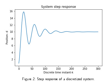
This is a typical response of an undamped system.

Next, we proceed with training the machine learning models. The following code defines a mass-spring model with arbitrary parameters and defines the discretization steps and the total number of time samples.

import numpy as np
import matplotlib.pyplot as plt

###############################################################################
#                   Model defintion
###############################################################################

# First, we need to define the system matrices of the state-space model:
# this is a continuous-time model, we will simulate it using the backward Euler method
A=np.matrix([[0, 1],[- 0.1, -0.000001]])
B=np.matrix([[0],[1]])
C=np.matrix([[1, 0]])

#define the number of time samples used for simulation and the discretization step (sampling)
time=200
sampling=0.5

To learn the model, we use a random input sequence. Furthermore, we use a random initial condition. Special care needs to be given to the definition of the training, validation, and test data. According to the Keras documentation, recurrent neural networks take a tensor input of the following shape: “(batch_size, timesteps, input_features)”. In our case, batch_size=1, timesteps=time+1, and input_features=2.
If we denote the test input data by “testX”, then the entry “testX[0,:,:]” has the following form

(10) $\begin{align*}\text{testX}[0,:,:]=\begin{bmatrix} x_{0}^{(1)} & x_{0}^{(2)} \\ u_{0} & 0 \\ u_{1} & 0 \\ \vdots & \vdots \\ u_{199} & 0 \end{bmatrix}\end{align*}$

First of all, in order to predict the system response, the model needs to “know” the initial state. This is why the first row of the above matrix is equal to the initial state.
The entries on the first column, starting from the row $2$ to the row $201$ are the input sequence (the force applied to the model). The corresponding entries on the second row are equal to zeros. This has been done in order to keep the sliced tensor dimension constant (Is there a better way to do this?). The output, denoted by “output_train” in the code, is defined in the same manner.
The output shape is (1,201,1). The first entry of the sliced output is $x_{01}$ and the remaining entries are equal to the observed output sequence.
Here for simplicity, we did not scale the training data. It should be emphasized that the inputs and outputs should not be scaled independently since they are related (special attention needs to be dedicated to the scaling or “detrending” problem).

For training, validation, and test data we use different initial states and input sequences. That is, for randomly generated input sequences and initial conditions, we simulate the system dynamics to obtain three different input-output data sets that are used for training, test, and validation. This data is then used to form the input and output tensors. To define the training data, we simulate the system only once. This is done because in real-life applications, it is time-consuming to observe the system dynamics for different inputs and initial conditions, and we often can do it only once by performing a single actuation and data collection experiment.
A Python code defining the training, validation, and test datasets, is given below.

###############################################################################
#                  Create the training data
###############################################################################
#define an input sequence for the simulation
input_seq_train=np.random.rand(time,1)
#define an initial state for simulation
x0_train=np.random.rand(2,1)


# here we simulate the dynamics
from backward_euler import simulate
state,output_train=simulate(A,B,C,x0_train,input_seq_train, time ,sampling)    

output_train=output_train.T
# this is the output data used for training
output_train=np.reshape(output_train,(1,output_train.shape[0],1))

input_seq_train=np.reshape(input_seq_train,(input_seq_train.shape[0],1))
tmp_train=np.concatenate((input_seq_train, np.zeros(shape=(input_seq_train.shape[0],1))), axis=1)
tmp_train=np.concatenate((x0_train.T,tmp_train), axis=0)
# this is the input data used for training
trainX=np.reshape(tmp_train, (1,tmp_train.shape[0],tmp_train.shape[1]))

###############################################################################
#               Create the validation data
###############################################################################
# new random input sequence
input_seq_validate=np.random.rand(time,1)
# new random initial condition
x0_validate=np.random.rand(2,1)

# create a new ouput sequence by simulating the system 
state_validate,output_validate=simulate(A,B,C,x0_validate,input_seq_validate, time ,sampling)    
output_validate=output_validate.T
# this is the output data used for validation
output_validate=np.reshape(output_validate,(1,output_validate.shape[0],1))

input_seq_validate=np.reshape(input_seq_validate,(input_seq_validate.shape[0],1))
tmp_validate=np.concatenate((input_seq_validate, np.zeros(shape=(input_seq_validate.shape[0],1))), axis=1)
tmp_validate=np.concatenate((x0_validate.T,tmp_validate), axis=0)
# this is the input data used for validation
validateX=np.reshape(tmp_validate, (1,tmp_validate.shape[0],tmp_validate.shape[1]))
###############################################################################
#               Create the test data
###############################################################################
# new random input sequence
input_seq_test=np.random.rand(time,1)
# new random initial condition
x0_test=np.random.rand(2,1)

# create a new ouput sequence by simulating the system 
state_test,output_test=simulate(A,B,C,x0_test,input_seq_test, time ,sampling)    
output_test=output_test.T
# this is the output data used for test
output_test=np.reshape(output_test,(1,output_test.shape[0],1))

input_seq_test=np.reshape(input_seq_test,(input_seq_test.shape[0],1))
tmp_test=np.concatenate((input_seq_test, np.zeros(shape=(input_seq_test.shape[0],1))), axis=1)
tmp_test=np.concatenate((x0_test.T,tmp_test), axis=0)
# this is the input data used for test
testX=np.reshape(tmp_test, (1,tmp_test.shape[0],tmp_test.shape[1]))

Next, we define the networks. We will compare three network architectures: SimpleRNN, GRU, and LSTM. For brevity, we do not explain these network architectures.
An interested reader is advised to consult the Keras documentation.

from keras.models import Sequential
from keras.layers import Dense
from keras.layers import GRU
from keras.layers import LSTM
from keras.layers import SimpleRNN
from keras.optimizers import RMSprop
from keras.layers import TimeDistributed
from keras.callbacks import ModelCheckpoint

model=Sequential()
#model.add(SimpleRNN(32, input_shape=(trainX.shape[1],trainX.shape[2]),return_sequences=True))
#model.add(GRU(32, input_shape=(trainX.shape[1],trainX.shape[2]),return_sequences=True))
model.add(LSTM(32, input_shape=(trainX.shape[1],trainX.shape[2]),return_sequences=True))
#model.add(Dense(1))
model.add(TimeDistributed(Dense(1)))  #there is no difference between this and model.add(Dense(1))...
# does not make sense to use metrics=['acc'], see https://stackoverflow.com/questions/41819457/zero-accuracy-training-a-neural-network-in-keras
model.compile(optimizer=RMSprop(), loss='mean_squared_error', metrics=['mse'])


# after every epoch, we save the model, this is the absolute path on my C: drive, so the path is
# C:\python_files\system_identification\models\
filepath="\\python_files\\system_identification\\models\\weights-{epoch:02d}-{val_loss:.6f}.hdf5"
checkpoint = ModelCheckpoint(filepath, monitor='val_loss', verbose=0, save_best_only=False, save_weights_only=False, mode='auto', period=1)
callbacks_list = [checkpoint]
history=model.fit(trainX, output_train , epochs=2000, batch_size=1, callbacks=callbacks_list, validation_data=(validateX,output_validate), verbose=2)


# load the model with the smallest validation loss
#model.load_weights("weights-1997-1.878475.hdf5")

# use the test data to predict the model response
testPredict = model.predict(testX)

A few comments about the code are in order. In code lines 11-13, we use the parameter “return_sequences=True”, because we want that the used RNN networks return the state sequence at every time sample (in total we have 201 time samples). Then, in code lines 22-24 we say to the compiler that we want to store the model (network parameters) after each epoch. The file names are
defined according to the validation loss. This has been done in order to retrieve the model with the smallest validation loss. This should be the “best” model, which should be tested using the test data. The commented line 29 loads the model with the best validation loss. In code line 32 we use the test data to generate the predicted output, which is then compared with the “true” test output obtained by simulating the original system.

The following code plots the predicted and “true” test data, and plots the training and validation losses with respect to the training epoch number.

###############################################################################
#  Plot the predicted and "true" output and plot training and validation losses
###############################################################################

# plot the predicted and the "true" (test) outputs
time_plot=range(1,time+2)
plt.figure()
plt.plot(time_plot,testPredict[0,:,0], label='Real output')
plt.plot(time_plot,output_test[0,:],'r', label='Predicted output')
plt.xlabel('Discrete time steps')
plt.ylabel('Output')
plt.legend()
plt.savefig('responseLSTM32.png')
plt.show()

loss=history.history['loss']
val_loss=history.history['val_loss']
epochs=range(1,len(loss)+1)
plt.figure()
plt.plot(epochs, loss,'b', label='Training loss')
plt.plot(epochs, val_loss,'r', label='Validation loss')
plt.title('Training and validation losses')
plt.xlabel('Epochs')
plt.ylabel('Loss')
plt.xscale('log')
#plt.yscale('log')
plt.legend()
plt.savefig('lossLSTM32.png')
plt.show()

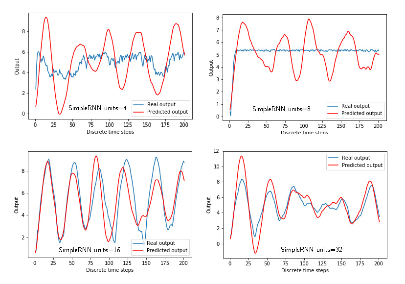
Figure 3 below shows the predicted and “true” outputs for the “simpleRNN” architecture for different numbers of units (4,8,16,32). The number of units is the first parameter in the definition of the recurrent layer:

model.add(SimpleRNN(units, input_shape=(trainX.shape[1],trainX.shape[2]),return_sequences=True))

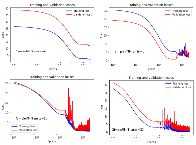
Figure 4 below shows the training and validation losses for the “simpleRNN” architecture for different numbers of units (4,8,16,32). The “simpleRNN” architecture with the largest number of units gives the best prediction. Here it should be noted that the training is stopped after 2000 epochs, and the effect of overfitting is not clearly visible.

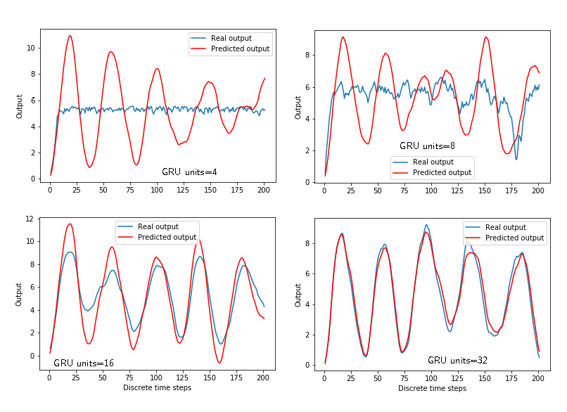
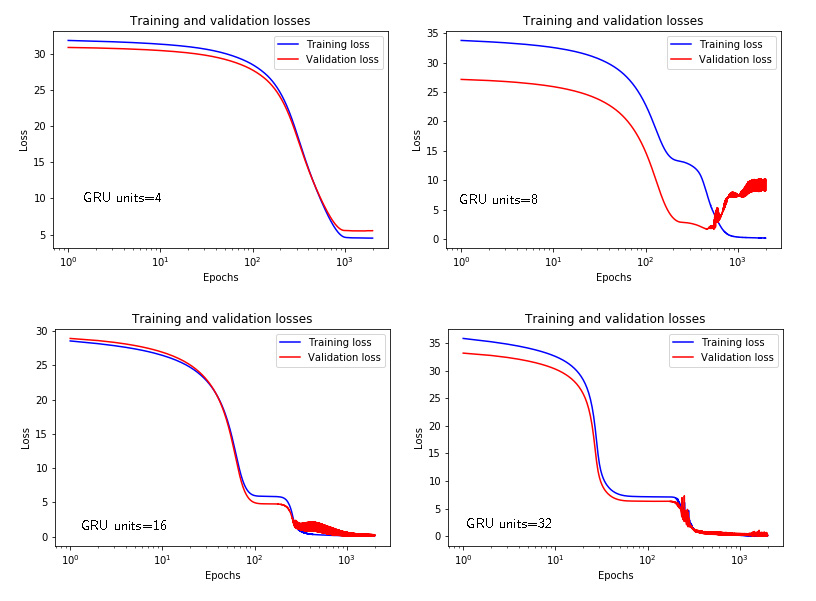
Figure 3: Predicted and “true” outputs of the “simpleRNN” architecture for different number of units.

Figure 4: Training and validation losses of the “simpleRNN” architecture for different number of units.

Similarly to Figs. 3 and 4, Figs. 5 and 6 show the time response and losses for the GRU networks with respect to the number of units.

Figure 5: Predicted and “true” outputs of the “GRU” architecture for different number of units.

Figure 6: Training and validation losses of the “GRU” architecture for different number of units.

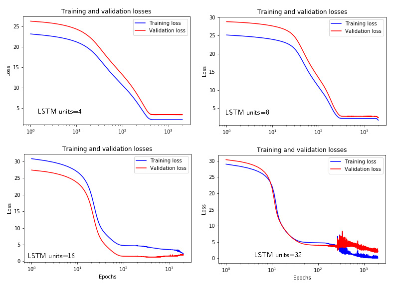
Figures 7 and 8 show the time response and losses for the LSTM networks with respect to the number of units.

Figure 7: Predicted and “true” outputs of the “LSTM” architecture for different number of units

Figure 8: Training and validation losses of the “LSTM” architecture for different number of units.

We can see that we need a relatively high number of units (that is, the model order) to estimate the model. This is due to the two issues. First of all, we need to increase the number of epochs to obtain better results. Secondly, since the model is linear, we need to tell to Keras that we want to use linear activation functions and that we do not need bias. The following code achieves this:

model=Sequential()
model.add(SimpleRNN(2, input_shape=(trainX.shape[1],trainX.shape[2]),use_bias=False, activation='linear',return_sequences=True))
#model.add(GRU(32, input_shape=(trainX.shape[1],trainX.shape[2]),return_sequences=True))
#model.add(LSTM(32, input_shape=(trainX.shape[1],trainX.shape[2]),return_sequences=True))
#model.add(Dense(1))

model.add(Dense(1, activation='linear', use_bias=False))
#model.add(TimeDistributed(Dense(1,activation="linear",use_bias=False)))  #there is no difference between this and model.add(Dense(1))...
# does not make sense to use metrics=['acc'], see https://stackoverflow.com/questions/41819457/zero-accuracy-training-a-neural-network-in-keras
model.compile(optimizer=RMSprop(), loss='mean_squared_error', metrics=['mse'])
# after every epoch, we save the model, this is the absolute path on my C: drive, so the path is
# C:\python_files\system_identification\models\
filepath="\\python_files\\system_identification\\models\\weights-{epoch:02d}-{val_loss:.6f}.hdf5"
checkpoint = ModelCheckpoint(filepath, monitor='val_loss', verbose=0, save_best_only=True, save_weights_only=False, mode='auto', period=1)
callbacks_list = [checkpoint]
history=model.fit(trainX, output_train , epochs=4000, batch_size=1, callbacks=callbacks_list, validation_data=(validateX,output_validate), verbose=2)

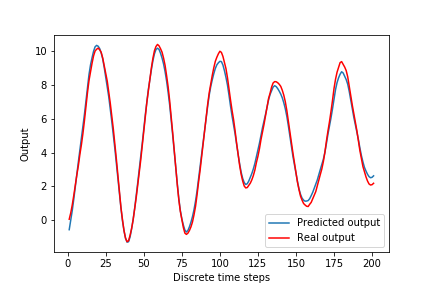
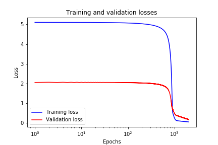
In code line 2 we specify a “SimpleRNN” with 2 units, we specify a linear activation function, and we set bias to “false”. Also, in code line 7 we specify that in the output layer we want to use linear activation function and that we do not want to use bias. The prediction performance of the modified model is given in Fig. 9 below, and training and validation losses are given in Fig. 10 below. Finally, in code line 16, we increase the number of epoch to 4000 to obtain better results.

Figure 9: The prediction performance for modified “SimpleRNN()”. Note that in this case we are using 2 units and epoch=4000.

Figure 10: *Training and validation losses for modified “SimpleRNN” architecture. Note that in this case we are using 2 units and epoch=4000.*

4. Critique, Conclusions, and Future Work

We have explained how to use Keras/TensorFlow library to reproduce an input-output behavior of a dynamical system.
The main drawback of the present approach is that we need to know an initial condition to apply it. In practice, it is rarely the case that we know the initial condition of the system. One of the ways to overcome this is to simply ignore the initial condition since if the system is stable, the effect of the initial condition will fade away as time increases. Another approach is to reformulate the model we want to estimate and to try to estimate the model in the autoregressive with exogenous input form. This model predicts the system output only on the basis of the past inputs and outputs.

1. Motivation

2. Problem Formulation

3. Numerical Example and Python Codes

4. Critique, Conclusions, and Future Work

admin

You might also like

Tutorial on How to Create URDF File and Model of 4-Wheeled Mobile Robot in ROS

Pole Placement Example 1- Design PID Controller to Achieve Desired Closed-Loop Behavior

Solve Differential Equations with Time-Varying Inputs and Coefficients in Python