Undamped Linear Harmonic Oscillator – Fusion of Engineering, Control, Coding, Machine Learning, and Science

In this lecture, we introduce the concept of harmonic oscillators. We derive an equation of motion of a harmonic oscillator and derive an analytical solution. Models of harmonic oscillators are archetypical models of a number of mechanical and electrical systems. A YouTube video accompanying this post is given below.

A basic example of a harmonic oscillator is a mass-spring system shown in Fig. 1 below.

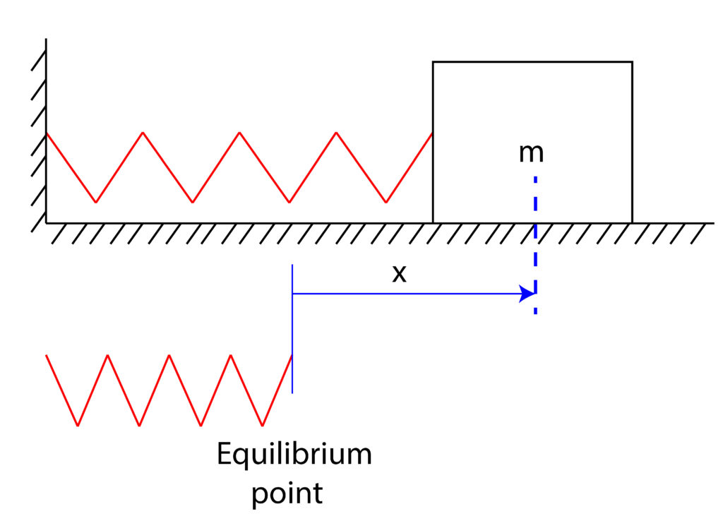
An object of a mass $m$ is attached to the wall by a spring with stiffness of $k$ . If we displace the object from its equilibrium position, the object will oscillate, and since there is no damping the object will oscillate forever. Our goal is to derive the equation describing the motion of the object as a function of time and to solve such an equation. As always, the first step is to derive a free-body diagram that is shown in Fig. 2 below. The equilibrium position is established for the displacement of $x=0$ for which the spring is not compressed or extended.

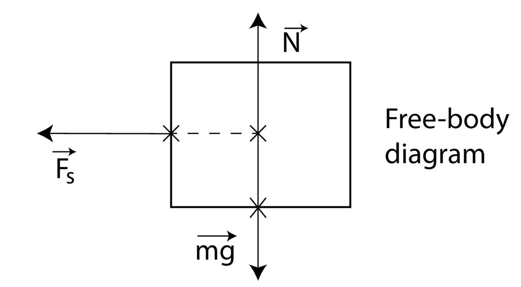
Figure 2: A free-body diagram of the object.

The force $\vec{F}_{s}$ is the spring force whose magnitude is equal to $-k x$ , where $x$ is the displacement of the object from its equilibrium position.

The next step is to apply Newton’s second law:

(1) $\begin{align*}m\vec{a}=\sum_{i=1}^{n=3} \vec{F}_{i}=\vec{F}_{s}+\vec{mg}+\vec{N}\end{align*}$

By projecting this equation onto the x-axis, we obtain:

(2) $\begin{align*}m\ddot{x}=-kx\end{align*}$

By defining $\omega_{n}=\sqrt{\frac{k}{m}}$ , we can write the last equation as follows:

(3) $\begin{align*}\ddot{x}+\omega_{n}^{2}x=0\end{align*}$

The equation (3) is the equation of motion describing the dynamics of the mass-spring system. For given initial conditions, the solution of this equation is a function

(4) $\begin{align*}x=x(t)\end{align*}$

The quantity $\omega_{n}=\sqrt{\frac{k}{m}}$ is the natural frequency. You will see later in this lecture why this quantity is called the natural frequency.
The next step is to solve the equation of motion. We assume a solution of the following form:

(5) $\begin{align*}\tilde{x}(t)=e^{st}\end{align*}$

where $s$ is a complex number. By substituting (5) in (3), we obtain

(6) $\begin{align*}s^{2} e^{st} + \omega_{n}^{2} e^{st} =0\end{align*}$

or compactly

(7) $\begin{align*}(s^{2}+\omega_{n}^{2}) e^{st} =0\end{align*}$

Since $e^{st}$ cannot be equal to zero, the only possibility is that

(8) $\begin{align*} s^{2}+\omega_{n}^{2} =0\end{align*}$

The equation (8) is called the auxiliary equation. The soluton of this equation is given by

(9) $\begin{align*}s_{1,2}=\pm \omega_{n} i\end{align*}$

where $i$ is the imaginary unit. Now, the solution can be written as follows:

(10) $\begin{align*}x(t)=C_{1}e^{i\omega_{n}t}+ C_{2}e^{-i\omega_{n}t} \end{align*}$

where $C_{1},C_{2}$ are constants. We want to get rid of the imaginary unit in the equation (10). This can be done by using the Euler’s formula:

(11) $\begin{align*}e^{\phi i}= cos(\phi)+i sin(\phi)\end{align*}$

where $\phi$ is an arbitrary real number. By applying this formula to (10), we obtain

(12) $\begin{align*}x(t)=C_{1}\big(cos(\omega_{n}t)+i sin(\omega_{n}t) \big)+C_{2} \big(cos(-\omega_{n}t)+i sin(-\omega_{n}t) \big)=\\x(t)= (C_{1}+C_{2}) cos( \omega_{n}t )+ i(C_{1}-C_{2}) sin( \omega_{n}t ) \end{align*}$

where we used the fact that $cos( -\omega_{n}t )= cos( \omega_{n}t )$ and $sin(- \omega_{n}t )= -sin(\omega_{n}t )$ . Finally by introducing new constants $K_{1}= (C_{1}+C_{2})$ and $K_{2}= i(C_{1}-C_{2})$ , we can write the equation (16) as follows:

(13) $\begin{align*}x(t)=K_{1} cos( \omega_{n}t ) +K_{2} sin( \omega_{n}t ) \end{align*}$

The equation (13) is the solution of the equation of motion (8). Our next goal is to write this equation in a more compact form. Namely, we want to write this equation as follows:

(14) $\begin{align*}x(t)=Asin(\omega_{n}t+\theta)\end{align*}$

where $A$ is the ampliture of oscillation and $\theta$ is the phase angle. We recall the addition formula:

(15) $\begin{align*}sin(\alpha +\beta)= sin(\alpha) cos(\beta)+sin(\beta)cos(\alpha)\end{align*}$

By applying this formula to (14), we obtain

(16) $\begin{align*}x(t)=A sin( \omega_{n}t )cos(\theta) + A sin( \theta )cos( \omega_{n}t ) \end{align*}$

By comparing (16) and (13), we obtain

(17) $\begin{align*}K_{1}= A sin( \theta ) ,\;\; K_{2}=Acos(\theta)\end{align*}$

From these two equations, we obtain:

(18) $\begin{align*}A=\sqrt{K_{1}^{2}+ K_{2}^{2} }, \theta=arctan(\frac{K_{1}}{K_{2}})\end{align*}$

The equation (14) is important since it tells us that the mass will oscillate with the angular frequency of $\omega_{n}$ , with the amplitude of $A$ , and with the phase of $\theta$ . The angular frequency $\omega_{n} = frac{2\pi}{T}=2\pi f$ , where $f$ is the frequency in $[Hz]$ and $T$ is the period. Since the angular frequency is our natural frequency, we see that the frequency of oscillation is determined by

(19) $\begin{align*}\frac{k}{m}\end{align*}$

That is, higher the stiffness and smaller the mass, higher is the frequency of oscillation and vice-versa. Also, the frequency of oscillation is independent from the initial condition. That is, the object will oscillate with a predetermined frequency that only depends on the mass and on the spring stiffness. This is the main reason why $\omega_{n}$ is called the natural frequency.

Now in order to find the constants, $K_{1},K_{2}$ or the amplitude and the phase, we need to include the initial conditions. Let us assume that at the time instant $t=0$ , the position of the object was at $x=0$ and that the velocity $\dot{x}_{0}$ is $\dot{x}_{0}=1$ . Let us substitute these initial conditions in the solution (13). We have

(20) $\begin{align*}x_{0}= K_{1} cos( \omega_{n} 0 ) +K_{2} sin( \omega_{n} 0 )=0 \\K_{1}=0 \end{align*}$

Substituting this value in (13) and differentiating, we obtain

(21) $\begin{align*}\dot{x}_{0}=K_{2}\omega_{n}cos( \omega_{n} 0)=1 \notag \\K_{2}=\frac{1}{\omega_{n}}\end{align*}$

So, the solution is

(22) $\begin{align*}x(t)=\frac{1}{\omega_{n}}sin(\omega_{n}t)\end{align*}$

admin

You might also like

Install MicroBlaze Processor and Start with C/C++ Coding FPGAs in Vivado and Vitis

Cart Pole Control Environment in OpenAI Gym (Gymnasium)- Introduction to OpenAI Gym

Analog-to-digital conversion in Raspberry Pi and temperature sensing – 3